Wavelet-Based Segmentation on the Sphere

WAVELET-BASED SEGMENTATION ON THE SPHERE

arXiv:1609.06500v1 [cs.CV] 21 Sep 2016

XIAOHAO CAI∗ , CHRISTOPHER G. R. WALLIS∗ , JENNIFER Y. H. CHAN∗ , AND JASON D. MCEWEN∗ Abstract. Segmentation is the process of identifying object outlines within images. There are a number of efficient algorithms for segmentation in Euclidean space that depend on the variational approach and partial differential equation modelling. Wavelets have been used successfully in various problems in image processing, including segmentation, inpainting, noise removal, super-resolution image restoration, and many others. Wavelets on the sphere have been developed to solve such problems for data defined on the sphere, which arise in numerous fields such as cosmology and geophysics. In this work, we propose a wavelet-based method to segment images on the sphere, accounting for the underlying geometry of spherical data. Our method is a direct extension of the tight-frame based segmentation method used to automatically identify tube-like structures such as blood vessels in medical imaging. It is compatible with any arbitrary type of wavelet frame defined on the sphere, such as axisymmetric wavelets, directional wavelets, curvelets, and hybrid wavelet constructions. Such an approach allows the desirable properties of wavelets to be naturally inherited in the segmentation process. In particular, directional wavelets and curvelets, which were designed to efficiently capture directional signal content, provide additional advantages in segmenting images containing prominent directional and curvilinear features. We present several numerical experiments, applying our wavelet-based segmentation method, as well as the common K-means method, on realworld spherical images, including an Earth topographic map, a light probe image, solar data-sets, and spherical retina images. These experiments demonstrate the superiority of our method and show that it is capable of segmenting different kinds of spherical images, including those with prominent directional features. Moreover, our algorithm is efficient with convergence usually within a few iterations. Key words. Image segmentation, Wavelets, Curvelets, Tight frame, Sphere.

1. Introduction. Spherical images are common in nature, for example, in cosmology [45,52,53], astrophysics [66], planetary science [5], geophysics [69], and neuroscience [61], where images are naturally defined on the sphere. Clearly, images defined on the sphere are different to Euclidean images in 2D and 3D in terms of symmetries, coordinate systems and metrics constructed (see for example [37, 71]). Image segmentation aims to separate a given image into different components, where each part shares similar characteristics in terms of, e.g., edges, intensities, colours, and textures. It generally serves as a preliminary step for object recognition and interpretation, and is a fundamental yet challenging task in image processing. In this paper, we present an effective segmentation method that uses spherical wavelets to segment spherical images. In the literature, many different approaches have been proposed for image segmentation for 2D, 3D and vector-valued images, e.g., [12–16,22–24,29,31,36,38,39,57, 68, 70, 73]. In particular, in [57] the well-known Mumford-Shah model was proposed, which formulates the image segmentation problem by minimising an energy function and finding optimal piecewise smooth approximations of the given image. More details about these kind of methods can be found in [8, 12, 13, 23, 24, 38]. These types of methods generally give good segmentation results. However, their applicabilities and performance heavily depend on the models used; in some cases (e.g. segmenting images containing complex textures) the models are difficult or expensive to compute due to the non-convex nature of the problem. In [68], a graph-cut based method was proposed to segment point clouds into different groups. The more pixels in the image, the larger the size of the eigenvalue problem need to be solved, which makes ∗ Mullard

Space Science Laboratory (MSSL), University College London (UCL), UK 1

the method inefficient in terms of speed and accuracy. Methods based on deformable models [29,39] segment via evolving geodesic active contours that are built from a partial differential equation, with the ability to detect twisted, convoluted and occluded structures, but are sensitive to noise and blur in images. Recently, segmentation methods [12, 13, 16, 22] designed utilising techniques in image restoration (e.g. [26, 59, 64]), were proposed for gray-scale images. In [12], a segmentation model that combines the image segmentation model of [57] and the data fidelity terms from image restoration models [26, 59, 64] was considered to deal with images contaminated by different types of noise (e.g. Gaussian, Poisson or impulsive noise). In [13, 22], the methodology of two-stage methods, solving image restoration models first followed by a thresholding second stage, was proposed. One advantage of these methods is the fast speed of implementation. The T-ROF method (thresholding the Rudin-Osher-Fatemi model) in [12] concluded that the thresholding approach for segmentation was equivalent to solving the Chan-Vese segmentation model [23]. In additional to the methods above, approaches based on wavelets and tight frames [6, 14, 15, 74] have been proposed for segmentation. In [14, 15], a tight-frame based segmentation method was designed for a vessel segmentation problem in medical imaging. The major advantage of this method is the ability to segment twisted, convoluted and occluded structures without user interactions. Moreover, the ability of the method to follow the branching of different layers, from thinner to larger structures, makes the method a good candidate for a tubular-structured segmentation problem in medical imaging. However, all the tight-frame systems discussed and used in [15] (e.g. framelets [62], contourlets [28], curvelets [21], and dual-tree complex wavelet [11]) are designed for 2D or 3D data on a Euclidean manifold. Consequently, these approaches cannot be applied to problems where data-sets live natively on the sphere. Wavelets have become a powerful analysis tool for spherical images, due to their ability to simultaneously extract both spectral and spatial information. A variety of wavelet frameworks have been constructed on the sphere in recent years, e.g. [2–4, 7, 9, 35, 40, 41, 43, 44, 47, 48, 50, 51, 55, 58, 65, 67, 72, 76, 77], and have led to many insightful scientific studies in the fields mentioned above (see [5, 53, 61, 66, 69]). Different types of wavelets on the sphere have been designed to probe different structure in spherical images, for example isotropic or directional and geometrical features, such as linear or curvilinear structures, to mention a few. Axisymmetric wavelets [7,35,40,58,72] are useful for probing spherical images with isotropic structure, directional wavelets [43, 47, 48, 51, 76] for probing directional structure, ridgelets [41, 56, 72] for analysing antipodal signals on the sphere, and curvelets [25,72] for studying highly anisotropic image content such as curve-like features (we refer to [17–20] for the general definition of Euclidean ridgelets and curvelets). Fast algorithms have been developed to compute exact forward and inverse wavelet transforms on the sphere for very large spherical images containing millions of pixels [46, 47, 51] (leveraging novel sampling theorems on the sphere [54] and the rotation group [42]). Localisation properties of wavelet constructions have also been studied in detail [7, 30, 43, 58, 60], showing important quasi-exponential localisation and asymptotic uncorrelation properties for certain wavelet constructions. An investigation into the use of axisymmetric and directional wavelets for sparse image reconstruction was performed recently in [75], showing excellent performance. The spherical wavelets adopted in the experimental section of this paper are reviewed briefly in Section 2. In this paper, we devise an iterative framework for segmenting spherical images 2

using wavelets defined on the sphere, extending the method proposed in [14, 15]. The first stage of the method, as a preprocessing step, suppresses noise in the given data by soft thresholding wavelet coefficients. Then, potential boundary pixels are classified gradually by the iterative procedure. The framework is compatible with any arbitrary type of spherical wavelet, such as the axisymmetric wavelets, directional wavelets, or curvelets mentioned above. The iterative strategy in the proposed framework is effective, particularly for images containing anisotropic textures. There is also flexibility regarding the implementation of iterations. Motivated by the two-stage methodology in [13, 16, 22], when segmenting images containing many (or mostly) isotropic structures, the iterative strategy in our method can be replaced by a simple thresholding to reduce the computation time significantly without sacrificing segmentation quality considerably. We test the proposed framework on a variety of types of spherical images, including an Earth topographic map, a light probe (spherical) image, two sets of solar data, and two retina images projected on the sphere. To the best of our knowledge, this is the first segmentation method that works directly on the whole sphere and is practical for any type of spherical images, benefiting from the compatibility of the method with any type of spherical wavelets. A method [63] was proposed for segmenting spherical particles in volumetric data sets based on an extension of the generalised Hough transform and an active contour approach. However, the data considered in [63] were 3D data containing spherical-like particles, not data defined on the sphere directly. The main contributions in this paper are: (1) a segmentation framework for spherical images is devised, for the first time; (2) the framework uses an iterative strategy with the flexibility to tailor the iterative procedure according to data types and features; (3) spherical wavelets, including axisymmetric wavelets, directional wavelets and the newly-constructed hybrid directional-curvelet wavelets, are implemented and tested in the framework; (4) a series of applications are presented, illustrating the performance of our proposed segmentation method. The remainder of this paper is organised as follows. In Section 2, we review related work about spherical wavelets and segmentation methods, and present our new hybrid directional-curvelet wavelet construction. In Section 3, we introduce our spherical segmentation method. In Section 4, the proposed method and methods for comparison are tested on a variety of spherical images such as an Earth map, light probe images, and two solar maps. To further demonstrate the ability of our method on segmenting highly directional and elongated structures, in Section 4 we also apply it to retinal images, which contain a complex network of blood vessels. Conclusions are given in Section 5. 2. Background. Let f ∈ L2 (S2 ) be the given image defined on the sphere S2 . Without loss of generality, we assume f in [0, 1]. Let ω = (θ, φ) ∈ S2 denote spher¯2 be the ical coordinates with colatitude θ ∈ [0, π] and longitude φ ∈ [0, 2π). Let S 2 discretised sphere of S . We review sampling, wavelets and discrete gradient operators on the sphere subsequently, before recalling the tight-frame based segmentation method of [14, 15]. In addition, we present a new hybrid directional-curvelet wavelet construction. 2.1. Sampling on the sphere. We adopt the equiangular sampling theorem on the sphere of [54], which defines how to capture the information content in a signal band-limited at L in ∼ 2L2 samples. This sampling theorem requires the fewest number of samples to capture all information content on band-limited spherical images. In additional, fast algorithms to perform the associated spherical harmonic 3

transform are presented [54]. Typically, we consider band-limited spherical images whose spherical harmonic coefficients f`m = 0, ∀` ≥ L, where f`m = hf, Y`m i and Y`m ∈ L2 (S2 ) are the spherical harmonics, with ` ∈ N and m ∈ Z satisfies |m| ≤ `. In practice many real-world signals can be approximated accurately by a band-limited signal). The equiangular sample positions of the sphere associated with this sampling theorem are given by θt =

π(2t + 1) , 2L − 1

φp =

2πp 2L − 1

where t ∈ {0, 1, . . . , L − 1} and p ∈ {0, 1, . . . , 2L − 2} index the equiangular samples in θ and φ, respectively. For example, when L = 512, the sphere is discretised with 512 × 1023 = 523776 samples. Please refer to [54] and references therein for more information about sampling on the sphere. 2.2. Wavelets on the sphere. In many real-life problems, data to be processed are usually in a discretised form, as described previously. Also, exact reconstruction of the signal is commonly desired. Scale-discretised wavelets [25,35,41,43,47,48,51,76] on the sphere allow the exact synthesis of discrete spherical images from their wavelet coefficients. We adopt scale-discretised wavelet constructions in this work, which we review concisely in this section. In addition, we present a new hybrid directionalcurvelet scale-discretised wavelet construction. Wavelet transforms. Let Ψ(j) ∈ L2 (S2 ) be the wavelet with wavelet scales j ∈ N and 0 ≤ Jmin ≤ j ≤ Jmax , which encode the angular localisation of Ψ(j) , where Jmin and Jmax are the minimum and maximum wavelet scales considered, respectively; see [47] for more details about j. For directional wavelet transforms, wavelet coefficients are defined on the rotation group SO(3), parameterised by Euler angles ρ = (α, β, γ) ∈ (j) SO(3) with α ∈ [0, 2π), β ∈ [0, π] and γ ∈ [0, 2π). Wavelet coefficients W Ψ ∈ 2 L (SO(3)) are computed by the wavelet forward transform (analysis) defined by Z (j) W Ψ (ρ) ≡ (f ~ Ψ(j) )(ρ) ≡ hf, Rρ Ψ(j) i = dΩ(ω)f (ω)(Rρ Ψ(j) )∗ (ω), (2.1) S2

where Rρ is a rotation operator related to a 3D rotation matrix Rρ by (Rρ Ψ(j) )(ω) ≡ ˆ ) (ˆ ω is the Cartesian vector of ω), dΩ(ω) = sin θdθdφ is the usual rotation Ψ(j) (Rρ-1 ω invariant measure on the sphere; the symbol h·, ·i, the operator ~, and ·∗ denote the inner product of functions, directional convolution on the sphere and complex conjugation, respectively. Low-frequency content of the signal not probed by wavelets are probed by the scaling function Φ ∈ L2 (S2 ), which is generally axisymmetric. The scaling coefficients W Φ ∈ L2 (S2 ) are given by Z W Φ (ω) ≡ (f Φ)(ω) ≡ hf, Rω Φi = dΩ(ω 0 )f (ω 0 )(Rω Φ)∗ (ω 0 ), (2.2) S2

where Rω = R(φ,θ,0) , and the operator denotes axisymmetric convolution on the sphere. The spherical image f can be synthesised perfectly from its wavelet and scaling coefficients (under the wavelet admissibility condition [47]) by the wavelet backward transform (synthesis) by Z JX max Z (j) f (ω) = dΩ(ω 0 )W Φ (ω 0 )(Rω0 Φ)(ω) + d%(ρ)W Ψ (ρ)(Rρ Ψ(j) )(ω), S2

j=Jmin

SO(3)

(2.3) 4

Fig. 2.1. Harmonic tilings of different types of wavelets, including axisymmetric wavelets, directional wavelets, and curvelets, respectively, from left to right (refer to [25]).

where d%(ρ) = sin βdαdβdγ is the usual invariant measure on SO(3). Construction of different types of wavelets. Spherical wavelets, constructed to ensure the admissibility condition is satisfied, are defined in harmonic space in the factorised form by r 2` + 1 (j) (j) κ (`)ζ`m , (2.4) Ψ`m ≡ 8π 2 where kernel κ(j) ∈ L2 (R+ ), a positive real function, is constructed to be a smooth function with compact support to control the angular localisation properties of wavelet (j) Ψ(j) , with harmonic coefficients Ψ`m = hΨ(j) , Y`m i; see [43] for the detailed definition. The directionality component ζ ∈ L2 (S2 ), with harmonic coefficients ζlm = hζ, Y`m i, is designed to control the directional localisation properties of Ψ(j) . The wavelets recovered are steerable when imposing an azimuthal band-limit N on the directionality component such that ζ`m = 0 for |m| ≥ N, ∀`, m. While steerability is achieved, the directional localisation of the wavelet is controlled by imposing a specific form for the directional auto-correlation of the wavelet. The detailed construction of ζ and ζ`m for directional wavelets can be found in [43] and those for curvelets can be found in [25]. In particular, the spherical curvelets proposed in [25] exhibits the parabolic scaling relation. Such a geometric feature is unique to curvelets, making it highly anisotropic and directionally sensitive, and thus suitable for extracting local curvilinear structures effectively. Moreover, scale-discretised wavelets support the exact analysis and synthesis of both scalar and spin signals, although only the former are considered herein. Fig. 2.1 and Fig. 2.2 show the harmonic tilings of different types of scale-discretised wavelets and the corresponding wavelets plotted on the sphere, respectively. We refer the reader to [35, 43, 47, 51, 76], and [25] for details about the construction of scalediscretised axisymmetric and directional wavelets, and curvelets, respectively. Code to compute these wavelet transforms is public and available in the existing S2LET1 package, which relies on the SSHT2 [54] and SO33 [42] packages. Hybrid wavelets. Different wavelet transforms have differing computational requirements. Generally, computing axisymmetric wavelet transforms are fastest with 1 http://www.s2let.org 2 http://www.spinsht.org 3 http://www.sothree.org

5

Axisymmetric wavelets

Directional wavelets (N = 5)

Directional wavelets (N = 6)

Curvelets

j=1

j=2

j=3

j=4

j=5

Fig. 2.2. Scalar scale-discretised axisymmetric wavelets, directional wavelets (N = 5 and 6), and curvelets on the sphere for L = 512, from the first row to the fourth row.

computational time scaling as O(L3 ) [35], directional wavelet transforms are slower with computational time scaling as O(N L3 ) [47], while curvelet transforms are the slowest with computational time scaling as O(L3 log2 L) [25]. As an example, a complete round-trip of a forward and backward wavelet transform, with band-limit L = 512, takes a few seconds on a Macbook with i5 processor for axisymmetric wavelets, several minutes for directional wavelets and several hours for curvelets (see Tables 4.1, 4.2, 4.3 and 4.4). However, the increase in computational cost is offset by an improved ability to represent directional and curvilinear structure for directional wavelets and curvelets, respectively. With the aim to exploit the advantages of the curvelet transform [25] while shortening the computational time needed, here we construct a hybrid form of wavelet transform on the sphere using both curvelets and directional wavelets. The idea (proposed as a future work in our paper [25]) is to describe small-scale features with directional wavelets and remaining features with curvelets, thereby inheriting the excellent directional localisation of curvelets and computational advantages of directional wavelets. The separation between the two wavelet types is performed in harmonic space, at a defined transition band-limit Ltrans . The curvelet transform is performed up to the band-limit Ltrans , ignoring the final wavelet scale. This provides the large-scale curvelet coefficients. In order to calculate the component of the image represented by 6

curvelets, the inverse transform is performed, yielding f curv . The directional wavelet coefficients are found by first subtracting this image from the original, f dir = f −f curv , before performing the directional wavelet transform on the difference image f dir . The balancing between curvelets and directional wavelets, Ltrans is also flexible and can be tuned in our hybrid construction, depending on the importance of directional structure in the image or the computational time available. This hybrid wavelet transform is implemented in the S2LET package.4 The current implementation is not optimised as it performs a full backward wavelet transform when only one scale needs to be transformed. This optimisation is left for future work. 2.3. Gradient operators on the sphere. The segmentation method devel∂f oped herein requires the computation of gradients on the sphere ∇f = ( ∂f ∂θ , ∂φ ), with the continuous magnitude of the gradient given by v ! !2 u u ∂f 2 1 ∂f t k∇f k ≡ + . ∂θ sin2 θ ∂φ Discrete gradient operators for the equiangular sampling scheme adopted [54] are defined in [49]. The discrete magnitude of the gradient is simply defined by s
2
2 1 δφ f . (2.5) k∇f k ≡ δθ f + 2 sin θt where δθ and δφ are finite difference operators. For more details of the discrete gradient operator please refer to [49]. 2.4. Tight-frame based segmentation method. The following presents the generic tight-frame algorithm used in e.g. [10]: 1

f (i+ 2 ) = U(f (i) ), f

(i+1)

T

= A Tλ (Af

(2.6) (i+ 12 )

),

i = 1, 2, . . . .

(2.7)

Here A and AT are the tight-frame (wavelets in our case) forward and backward transforms respectively, f (i) is an approximate solution at the i-th iteration, U is a problem-dependent operator (e.g. U is the identity operator for a denoising problem), and Tλ (·) is the soft-thresholding operator defined by Tλ (~v ) ≡ [tλ (v1 ), · · · , tλ (vn )]T , where ~v = [v1 , · · · , vn ]T ∈ Rn and λ ∈ R+ are a given vector and constant respectively, and  sign(vk )(|vk | − λ), if |vk | > λ, tλ (vk ) ≡ (2.8) 0, if |vk | ≤ λ. To obtain a binary result, where values 1 and 0 represent the object of interest and the background respectively, an iterative procedure was proposed in [14, 15] to gradually update an interval that contains pixel values of potential boundary pixels 4 Support for hybrid wavelets in the S2LET package will be made public following the publication of this article.

7

until the interval is empty. Note that the test image discussed in [14, 15] is assumed to have a low noise level and scaled to the range [0, 1]. The main segmentation procedures of [15] are as follows. Firstly, separate the given image to three parts by thresholding, i.e., area of background, area of object of interest, and the uncertainty-area which needs to be labelled as background or object in future steps. Secondly, denoise and smooth the uncertainty-area by the tight-frame algorithm [10] to get a new uncertainty-area which is smaller than the previous one. Thirdly, stop the algorithm when the uncertainty-area is empty (a binary result is then obtained), otherwise continue. 3. Spherical segmentation method. In [14, 15], the tight-frame based segmentation method is applied to Euclidean images but it is in principle extendable to a spherical domain and is compatible with different types of wavelets transforms. In this paper, the proposed wavelet-based segmentation framework on the sphere is a direct extension of the method [14, 15] to spherical images. The idea behind the method is to detect the candidates of possible pixels on (near) the boundary first, then gradually purify these boundary-like pixels via an iterative procedure until all pixels on the sphere are classified as inside or outside of a boundary. With the aid of the fact that possible pixels on the boundary have particular properties in terms of pixel values and gradients, boundary-like pixels are detected and represented by a range [a0 , b0 ]. Then, an iterative strategy shrinking this range is applied, so to keep removing pixels from it until the range itself is empty. All pixels are eventually classified either as in the foreground (the objects of interest) or in the background. Note that pixels in the foreground and in the background are represented respectively by values 1 and 0. When a binary result is obtained the algorithm stops. The greater the anisotropic structure in the image, the more complicated the boundary-like pixels in [a0 , b0 ]. Therefore, using an iterative procedure is particularly useful for images containing anisotropic structures. Otherwise, replacing the iterative procedure by thresholding is more economical (as demonstrated very effective in [13, 16, 22]). In the following, we discuss each of the iterative steps of the method in more detail. Preprocessing. If f is contaminated with significant noise, a preprocessing step to suppress the noise is necessary. We use one iteration step of the tight-frame algorithm (2.7) to deal with the noise by soft thresholding, i.e. f¯ = AT Tλ¯ (Af ).

(3.1)

Note that A here is a wavelet transform on sphere. Initialisation. Let Λ(0) be the initial set of potential boundary pixels, which is identified by using the gradient of f¯, i.e. pixels with gradient larger than a given threshold  are in Λ(0) , therefore ¯2 | k[∇f¯]k k1 > }. Λ(0) ≡ {k ∈ S

(3.2)

Here [∇f¯]k (cf. (2.5)) is the discrete gradient of f¯ at the k-th pixel on the sphere. Set f (0) = f¯, with Λ(0) defined in (3.2). We start the iterative process from i = 0. The i-th iteration is described in detail below. Step 1: computing the range [ai , bi ]. Given Λ(i) , define [ai , bi ] by ) ( ) ( (i) (i) µ(i) + µ+ µ(i) + µ− , 0 , bi ≡ min ,1 , (3.3) ai ≡ max 2 2 8

where µ(i) =

X (i) 1 fk (i) |Λ | (i)

(3.4)

k∈Λ

(i)

is the mean pixel value on Λ(i) , | · | denotes the cardinality of the set, fk is the pixel (i) (i) value of pixel k in spherical image f (i) , and µ− and µ+ are defined by (i) f (i) {k∈Λ(i) :fk ≤µ(i) } k , (i) |{k ∈ Λ(i) : fk ≤ µ(i) }|

P

(i) µ−

(i)

=

(i) f (i) {k∈Λ(i) :fk ≥µ(i) } k . (i) |{k ∈ Λ(i) : fk ≥ µ(i) }|

P

(i) µ+

=

(3.5)

(i)

Note that µ− and µ+ , the mean pixel values of the two sets separated by µ(i) , reflect the mean energies of the pixels on the boundary closer to the background and closer to the foreground respectively. The definition of [ai , bi ] in (3.3) is approximately half length of [ai−1 , bi−1 ], ensuring the shrinkage property of these ranges. Step 2: thresholding the image into three parts. Using [ai , bi ] ⊆ [0, 1], we separate image f (i) into three parts — those below (set those pixel values that are smaller than ai to 0), inside (stretch those pixel values between 0 and 1 using a simple linear contrast stretch), and above (set those pixel values that are larger than bi to 1) the range, i.e.,  (i) if fk ≤ ai ,   0,(i) 1 (i+ ) fk −mi (i) ¯2 . (3.6) fk 2 = ai ≤ fk ≤ bi , for all k ∈ S Mi −mi ,   (i) 1, if bi ≤ fk , where (i)

(i)

(i)

(i)

Mi = max{fk | ai ≤ fk ≤ bi , k ∈ Λ(i) }, mi = min{fk | ai ≤ fk ≤ bi , k ∈ Λ(i) }.

(3.7)

The set of the remaining pixels that wait to be labelled is represented by (i+ 21 )

Λ(i+1) = {k | 0 < fk

¯2 }. < 1, k ∈ S

(i+ 1 )

(3.8)

Note that if Λ(i+1) = ∅, the threshold image fk 2 is binary and the algorithm stops. Remark 3.1. After obtaining Λ(i+1) from formula (3.8), the segmentation accuracy could be improved by making a correction of Λ(i+1) , such as by adding the labelled but isolated (or wrongly labelled) pixels back to Λ(i+1) before moving to step (3.10) (or step (3.9)). We leave this to future work. When the pixels in range [ai , bi ] can be classified easily (e.g. the number of pixels left to be classified is few therefore they are no longer critical to the final segmentation result) as the background or the objects of interest, the thresholding step for segmentation can be invoked: ( (i+ 1 ) X 0, if fk 2 < µ, 1 (i+ 32 ) (i) µ = (i+1) fk = fk (3.9) (i+ 12 ) |Λ | 1, if f ≥ µ, (i+1) k

k∈Λ

and the iteration terminates. 9

Step 3: spherical wavelets iteration. Let I be the identity operator and P (i+1) be the operator where the entry is 1 if the corresponding index is in Λ(i+1) , and 0 otherwise. Then 1

1

f (i+1) ≡ (I − P (i+1) )f (i+ 2 ) + P (i+1) AT Tλ (Af (i+ 2 ) ).

(3.10)

Recall A here represents a wavelet transform on sphere (e.g. axisymmetric wavelets, directional wavelets, curvelets, or hybrid wavelets). Note that the values of all pixels outside Λ(i+1) are either 0 or 1, hence the cost of (3.10) can be reduced significantly by applying the forward and backward wavelet transforms on pixels around Λ(i+1) only. This optimisation is left for future work. 1 Stopping criterion. As soon as all the pixels of f (i+ 2 ) are either of value 0 or 1, or (i) equivalently when Λ = ∅, the iteration is terminated, then all the pixels with value 1 constitute the objects of interest otherwise they are considered as background. Algorithm 1 below summarises the steps required to segment a spherical image f by our segmentation method. Its convergence proof follows the proof given in [15]. In subsequent sections, algorithm 1 is referred to as WSSA for simplicity. Algorithm 1: Wavelet-based Spherical Segmentation Algorithm (WSSA) 1 2 3 4 5 6 7 8 9 10 11

Input: given image f ∈ L2 (S2 ) Preprocessing by (3.1) Set f (0) = f¯ and Λ(0) by (3.2) do compute [ai , bi ] by (3.3) 1 compute f (i+ 2 ) by (3.6) 1 stop if f (i+ 2 ) is a binary image compute Λ(i+1) by (3.8) 3 compute f (i+1) by (3.10) (or compute f (i+ 2 ) by (3.9) then stop) i=i+1 while Stopping criterion is not reached ;

4. Experiments. We apply our method, namely WSSA, to various kinds of real-life images, including an Earth topographic map, light probe image, solar datasets, and retina images projected on the sphere. Axisymmetric wavelets, directional wavelets, and hybrid wavelets constructed by combining the directional wavelets and curvelets are tested and their performances are compared. Algorithm 1 (WSSA) equipped with axisymmetric wavelets, directional wavelets and hybrid wavelets are referred to as WSSA-A, WSSA-D, and WSSA-H, respectively. The code to perform these spherical wavelets transforms used are available in the software package S2LET [35, 47]. The popular K-means method (e.g. [32, 34]) is implemented for comparison purposes. Here, the K-means method is applied to data on the sphere according to the pixels intensities, using the Matlab built-in function kmeans. All the experiments are executed on a MacBook with 2.2 GHz Intel Core i7 processor and 16GB RAM. Parameters. We set the spherical wavelet band-limit L = 512, the minimum angular scale Jmin = 2, and the number of directions probed by directional wavelets to be N = 5 and 6. We discretise the sphere S2 with size 512 × 1023 (refer to section ¯2 | = 523776. For the hybrid wavelets Ltrans ∈ {32, 64}, which means 2.1), therefore |S that curvelets are used for bands up to ` . {32, 64} and directional wavelets for the 10

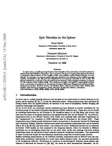
Test data

(a) noisy image

(b) noisy image

(c) noisy image

(d) original image

Segmentation results

(e) K-means

(f) WSSA-A

(g) WSSA-D

(h) WSSA-H

Fig. 4.1. Results of the Earth topographic map. First row: noisy image shown on the sphere (a) and in 2D using a mollweide projection (b), and the zoomed-in red rectangle area of the noisy (c) and original images (d), respectively; Second to fourth rows from left to right: results of methods K-means (e), WSSA-A (f ), WSSA-D (g) with N = 5 (odd N ), and WSSA-H (h), respectively.

remaining bands. Gaussian noise with standard deviation σ = kf k∞ 10−SNR/20 and 0 mean is added to the test data, where SNR = 30 dB and k · k∞ is the infinity norm ¯ = σ/4 in (referring to the maximum value). We fix the thresholding parameter λ (3.1) for denoising, and λ = σ/100 in (3.10) for segmentation during the spherical wavelet iterations. 4.1. Earth topographic map, light probe image and solar data-sets. Our first example is segmenting an Earth topographic map. The original Earth topography data are taken from the Earth Gravitational Model (EGM2008) publicly released by the U.S. National Geospatial-Intelligence Agency (NGA) EGM Development Team.5 The signal is band limited to L = 512 by performing a forward spherical harmonic transform, band limiting in harmonic space and transforming the signal back from its coefficients. Fig. 4.1 shows the results of the K-means and our WSSA (-A, -D, and -H) method 5 These data were downloaded and extracted using the tools available from Frederik Simons’ webpage: http://www.frederik.net.

11

Table 4.1 Earth map in Fig. 4.1: Number of unclassified points at each iteration and computation time in seconds. ∗ The fourth and fifth columns represent the results of WSSA-D with N = 5 and 6, respectively.

¯2

|S | |Λ(0) | |Λ(1) | |Λ(2) | |Λ(3) | |Λ(4) | |Λ(5) | |Λ(6) | |Λ(7) | |Λ(8) | |Λ(9) | |Λ(10) | |Λ(11) | Time

K-means 523776