Weather prediction with multiclass support vector ... - IEEE Xplore

520

IEEE/CAA JOURNAL OF AUTOMATICA SINICA, VOL. 4, NO. 3, JULY 2017

Weather Prediction With Multiclass Support Vector Machines in the Fault Detection of Photovoltaic System Wenying Zhang, Huaguang Zhang, Fellow, IEEE, Jinhai Liu, Kai Li, Dongsheng Yang, and Hui Tian

Abstract—Since the efficiency of photovoltaic (PV) power is closely related to the weather, many PV enterprises install weather instruments to monitor the working state of the PV power system. With the development of the soft measurement technology, the instrumental method seems obsolete and involves high cost. This paper proposes a novel method for predicting the types of weather based on the PV power data and partial meteorological data. By this method, the weather types are deduced by data analysis, instead of weather instrument. A better fault detection is obtained by using the support vector machines (SVM) and comparing the predicted and the actual weather. The model of the weather prediction is established by a direct SVM for training multiclass predictors. Although SVM is suitable for classification, the classified results depend on the type of the kernel, the parameters of the kernel, and the soft margin coefficient, which are difficult to choose. In this paper, these parameters are optimized by particle swarm optimization (PSO) algorithm in anticipation of good prediction results can be achieved. Prediction results show that this method is feasible and effective. Index Terms—Fault detection, multiclass support vector machines, photovoltaic power system, particle swarm optimization (PSO), weather prediction.

I. I NTRODUCTION

A

S the non-renewable energy brought about a series of problems such as air pollution, acid rain, greenhouse effect and etc., the importance of utilizing the clean and renewable energy is realized by more and more people. The photovoltaic (PV) power is a focus of wide attention by its distinct advantages such as safe, no noise, no pollution emission, short construction period, not constrained by the territory and so on [1]−[4]. Although PV power has many Manuscript received November 12, 2015; accepted April 9, 2016. This work was supported by the National Natural Science Foundation of China (61433004, 61473069) and IAPI Fundamental Research Funds (2013ZCX14). It was also supported by the Development Project of Key Laboratory of Liaoning Province, the Enterprise Postdoctoral Fund Projects of Liaoning Province. Recommended by Associate Editor Dianwei Qian. (Corresponding author: Huaguang Zhang.) Citation: W. Y. Zhang, H. G. Zhang, J. H. Liu, K. Li, D. S. Yang, and H. Tian, “Weather prediction with multiclass support vector machines in the fault detection of photovoltaic system,” IEEE/CAA J. of Autom. Sinica, vol. 4, no. 3, pp. 520−525, Jul. 2017. W. Y. Zhang is with the College of Science, Harbin Engineering University, Harbin 15001, China (e-mail: shuxue [email protected]). H. G. Zhang, J. H. Liu, K. Li, D. S. Yang, and H. Tian are with the College of Information, Northeastern University, Shenyang 110819, China (e-mail: [email protected]; [email protected]; [email protected]; [email protected]; [email protected]). Color versions of one or more of the figures in this paper are available online at http://ieeexplore.ieee.org. Digital Object Identifier 10.1109/JAS.2017.7510562

advantages, its power output is closely related to the weather condition. Usually, there are some differences between the local region weather forecast and the overall. In order to monitor the working state of the PV power system, a lot of PV enterprises install weather instruments to forecast the weather condition. According to a lots of meteorological data and the PV power data, the working state of the PV power system is judged by the experience of the power station staff. For example, when the meteorological data shows that the weather is sunny meanwhile the output power is very low, it means that the PV power system might have some faults, that is, the solar panels might be damaged or might have some unknown obstructions. This traditional method involves a lot of human factors. In addition, the weather instrument is expensive and its installation is inconvenient. Since the PV power outputs are closely related to the weather condition, we can utilize the PV output data and a part of weather data to predict the condition of the weather. With the development of the technology of big data, the weather instrument can be replaced by the soft measurement technology. In the data mining technologies, support vector machines (SVM) and neural network (NN) are two main intelligent methods. The optimization goal of NN is based on empirical risk minimization while the goal of SVM is based on structural risk minimization. Research results shown that compared with NN, the generalization quality of SVM is better and the algorithm of SVM has the global optimality [5]−[8]. Some researchers predicted the power of the PV power station using SVM [9]−[11]. Zhang et al. [12] utilized the air temperature, seasonal and day pattern, relative humidity and solar radiation as input in Least Square Support Vector Machine (LS-SVM) for the prediction of the short-term PV power output. Shi et al. [13] divided the weather conditions into four types. A one-day-ahead PV power output forecasting model for a single station is derived based on the weather forecasting data, the actual historical power output data, and the principle of SVM. R. De Leone [14] used historical data of solar irradiance, environmental temperature and past energy production to predict the PV energy production for the next day with an interval of 15 min. The technique used is based on m-SVR. From the above, it can be seen that many researchers use historical PV power output data and the meteorological data to predict the current PV power output by SVM, so it is feasible to predict the current weather types by the historical PV power output data and the historical meteorological data in

ZHANG et al.: WEATHER PREDICTION WITH MULTICLASS SUPPORT VECTOR MACHINES · · ·

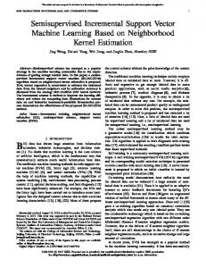
different weather types. According to the references, no article mentioned this direction up to now. Fig. 1 is a framework that can predict the types of weather with SVM.

521

F : X → Y that maps an instance x ¯ to an element y of Y . A framework that uses classifiers of the form is k

¯r · x FM (¯ x) = max{M ¯} r=1

¯ r is the where M is a matrix of size k × n over R and M rth row of M . The predicted label is the index of the row attaining the highest similarity score with x ¯. The optimization problem is m

min M,ξ

Fig. 1. Framework to predict the types of weather with SVM.

In this paper, the condition of weather is classified as three types, that is, sunny, foggy, cloudy or rainy, and the foggy means soft foggy or hazy, and the cloudy means heavy foggy or heavy hazy. We established the prediction model of each weather type at different times based on the data in normal working state of the PV power station. When the predicted weather type is different from the actual type, the PV power system may have faults. Our highlights are as follows: 1) We propose a model of multiclass SVM to predict the types of weather in the PV power system. It can replace weather measurement and monitoring system and save a lot of purchasing cost; 2) A better fault detection is obtained by using this SVM and comparing the predicted and the actual weather, instead of the traditional human experience; 3) The multiclass SVM in this paper is based on a direct method for training multiclass predictors and the parameters of the SVM model are optimized by PSO algorithm with the aim of achieving higher precision of classification. This paper is organized as follows: the multiclass SVM model based on a direct method for training multiclass predictors is presented in Section II. The output characteristics of PV power system and the data preprocessing are expressed in Section III. The intelligent optimization algorithm of PSO, which is used to optimize the parameters in the SVM model, is presented in Section IV. Forecasting results and discussions are given in Section V.

II. M ULTICLASS S UPPORT V ECTOR M ACHINES The basic idea of SVM is applied to binary classification. Most of the previous approaches are the method that decompose a multiclass problem into multiple independent binary classification tasks. In practice, these methods usually bring about the inseparable cases which will reduce the accuracy of classification. In order to obtain higher precision of classification, we use a direct method for training multiclass predictors [15]. Let S = {(¯ x1 , y1 ), . . . , (¯ xm , ym )} be a set of m training examples. We assume that each example x ¯i is drawn from a domain X ⊆ Rn and that each label yi is an integer from the set Y = {y1 , . . . , yk }. A multiclass classifier is a function

X 1 ξi c k M k22 + 2 i=1

¯y · x ¯r · x s. t. ∀i, r, M ¯i + δyi ,r − M ¯i ≥ 1 − ξi i P 2 where k M k22 = i,j Mi,j , c > 0 is a regularization constant, δyi ,r is equal to 1 if yi = r and 0 otherwise. The Lagrangian of the optimization problem is m

X X 1 X k M¯ r k22 + ξi + η i,r L (M, ξ, η) = c 2 r i=1 i,r ¯ r · x¯i − M ¯ y · x¯i − δ y ,r + 1 − ξi ] × [M i i s. t. ∀i, r, ηi,r ≥ 0. (1) Then, we obtain the following objective function of the dual program X 1X (¯ xi · x ¯j ) (¯ τi · τ¯j ) + c τ¯i · I¯yi maxQ (τ ) = − τ 2 i,j i s. t. ∀i, τ¯i ≤ I¯yi and ∀i, τ¯i · I¯ = 0.

(2)

Let I¯i be the vector whose components are all zero except for the ith component which is equal to one, and I¯ be the vector whose components are all one, and let τ¯i = I¯yi − η¯i . The classifier F (¯ x) becomes ( ) X ª k © k ¯ F (¯ x) = arg max Mr · x ¯ = arg max τ i,r (¯ xi · x ¯) . r=1

r=1

i

(3) The dual program and the resulting classifier depend only on inner products of the form (¯ xi · x ¯). Therefore, we can perform inner-product calculations in some high dimensional inner-product space with a kernel function K (·, ·) that satisfies Mercer’s conditions [16]. From (3), the general dual program using kernel functions is X 1X max Q (τ ) = − K (¯ xi , x ¯j ) (¯ τi · τ¯j ) + c τ¯i · I¯yi (4) τ 2 i,j i subject to ∀i, τ¯i ≤ I¯yi and ∀i, τ¯i · I¯ = 0 and the classification rule F (¯ x) becomes ( ) X k F (¯ x) = arg max τ i,r K (¯ xi , x ¯) . (5) r=1

i

The common kernels are shown as Table I, where the dot denotes the inner-product operation in Euclidean space, d is the degree of polynomial kernel, and σ is a constant parameter determining the width of RBF kernel. Different learning machines with various types of decision surfaces can be constructed by various kinds of kernel functions K (x, xi ).

522


In actual applications, it is important to select the proper kernel function and parameters in the SVM model.

C. Reconstruction of Data Based on Principal Component Analysis (PCA)

TABLE I K ERNEL F UNCTIONS

Since the collected data may have some correlation, they should be preprocessed by principal component analysis (PCA). The main process of PCA is to search the best orthogonal vectors to represent the data. These vectors are viewed as the basis of the normalized input data. Each orthogonal vector is perpendicular to the others. We call these vectors the principal components.

Name Linear Homogeneous polynomial Non-homogeneous polynomial RBF

Kernel function K (x, xi ) = x · xi K (x, xi ) = (x · xi )d K (x, xi ) = (1 µ + x · xi )d¶ K (x, xi ) = exp

−kM k2 2 2σ 2

III. PV P OWER S YSTEM O UTPUT C HARACTERISTICS AND DATA P REPROCESSING A. PV Power System Output Characteristics PV power output is unsteady and fluctuates along with the types of weather. The efficiency of the PV system can be expressed as [13]: η = η0 × [1 − γ (Tt − Tγ )] where Tt is temperature temperature; teries where 0.005 ◦ C−1 .

(6)

the temperature at time t; Tγ is the reference (298 K); η0 is the efficiency under reference γ is the temperature coefficient of solar batthe value is normally between 0.003 ◦ C−1 and The power output at time t is shown as P =I ×A×η

(7)

where A is the PV area (m2 ); η is the rating efficiency; I is radiation intensity of the PV inclined plane (kW/m2 ). From these equations, we know that there are some uncertain and varying parameters in the equations, and the factors, such as different solar panels, season, geographical location, weather, solar hour angle, observation date, time and clouds are all closely connected with these parameters. Consequently, many factors will affect the efficiency of the PV power system. In addition to the PV power output data, we selected a part of meteorological data as our input data. The input variables include atmospheric temperature, solar irradiance, time, electric current, power, voltage, dew point temperature and relative humidity. Our data was collected from a small PV power station in Shenyang city, which is located in the northeast of China. We collected the data covering the month of May. The data was measured hourly from 6 a.m. to 6 p.m. , including 365 effective samples. All the cases are measured in the normal working states. We selected 215 samples for training the SVM model and the others for testing the model. B. Normalization When the dimensions of variables are not consistent, the situation that larger number swallows smaller number often happens. If the data is preprocessed into a fixed range before it is input into the SVM model, the above situation will hardly happen. In this paper, we let the data be restricted within the range from 0 to 50. The process formula is shown as xi − xmin × 50 χi = xmax − xmin where xi is the original input data, and xmax and xmin are the maximum and minimum input data, respectively.

IV. O PTIMIZING THE PARAMETERS IN M ULTICLASS SVM SVM is suitable for classification, but the classified results depend on the type of the kernel, the parameters of the kernel, and the soft margin coefficient, which are difficult to choose. Particle swarm optimization (PSO) algorithm is suitable for solving this problem. It is based on the birds flocking behavior [17]. In PSO algorithm, particles, without quality and volume, fly through a D-dimensional space, adjusting their positions in the D-dimensional space according to their own or their neighbors experiences. The position of the particle i is represented with a position vector Xi (k) = (xi1 (k) , xi2 (k) , . . . , xiD (k)) and a velocity vector Vi (k) = (vi1 (k) , vi2 (k) , . . . , viD (k)). The best personal position that particle i has visited shows as Pi (k) = (pi1 (k) , pi2 (k) , . . . , piD (k)). The best global position that all particles have visited shows as Pg (k) = (pg1 (k) , pg2 (k) , . . . , pgD (k)). The particle’s position and speed are continuous real numbers. In every time step k, particle i changes its velocity and position according to the following equations: vid (k + 1) = ωvid (k) + η1 λ1 (pid (k) − xid (k)) + η2 λ2 (pgd (k) − xid (k))

(8)

xid (k + 1) = xid (k) + vid (k + 1)

(9)

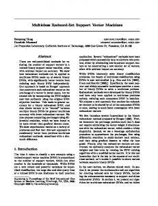
where 1 ≤ i ≤ m, 1 ≤ d ≤ D, λ1 , λ2 are the uniform random numbers, η1 and η2 are the positive acceleration coefficients, respectively. In this paper, let the fitness function of PSO be the objective function of SVM and the fitness value be the error of training, and the number of particles is 5. The dimension of the particle is 2, and they represent parameter σ in the RBF kernel function and the soft margin coefficient c, respectively. Set ω = 1, η 1 = η 2 = 1.5. The range of σ, c, and v id (k) is between 10−2 and 102 . From Fig. 2, we can see that the results of iteration have no change after about 55 generations. Then, we get the best parameters σ = 4.35, c = 66.205. The algorithm procedure is given as follows: Step 1: Initialize all particles including the initial positions and speeds; Step 2: Calculate the fitness value of each particle i; Step 3: For each particle, update Pi (k) and Pg (k) according to the fitness values; Step 4: After each update of parameter c, initialize it by the probability of 0.1 to make the particles out of the previous optimal value and search in a larger space;


Fig. 2. Curve of fitness values in PSO.

Step 5: Update Xi (k) and Vi (k) according to the (8) and (9); Step 6: When reach the maximal times of generation that we set before, the program is terminated. V. F ORECASTING R ESULTS AND D ISCUSSIONS For the unsteady, periodic and nonlinear relationship between the input variables and the output variables, we present multiclass SVM model for predicting the types of weather. The variables that preprocessed by PCA are viewed as the final input of the SVM model for training. The types of weather, which is sunny, foggy, cloudy or rainy, are viewed as the output of the SVM model. The training set and the testing set are shown in Table II.

523

other samples. The homogeneous polynomial kernel function has higher accuracy in foggy samples but lower accuracy in the other samples. The non-homogeneous polynomial kernel function has higher accuracy in sunny samples, and has lower accuracy in the other samples. Thus, the RBF kernel is suitable for this question. Its training time is shorter and its accuracy is higher. We took three principal components whose total contribution rate was over 85 %. The principal components have no physical meanings, because each principal component (PC) is a linear combination of some input variables. The testing samples expressed by three principal components are shown in Fig. 4. After prediction based on multiclass SVM with RBF kernel, they are shown in Fig. 5. We can see that the sunny samples almost have no change, except for few samples. For example, a few points in Fig. 4 have changed their identification marks, which are shown in Fig. 5. This leads to the error of classification. The number of changed identification marks in the cloudy or rainy samples is very small. Compared with the others, the number of changed identification marks in the foggy samples is the most.

TABLE II T RAINING S ET AND T ESTING S ET OF S AMPLES

Training set Testing set

Sunny samples 153 104

Foggy samples 36 25

Cloudy or rainy samples 26 21

Total samples 215 150

Fig. 3 shows that there exists relations between the output power of the PV power system and the types of weather. The relations are not linearly separable. SVM is adaptable to dealing with the nonlinear situation, while the traditional methods usually do not work in such situation.

Fig. 3. Relations between the output power and the types of weather.

Table III shows that the linear kernel function has higher accuracy in cloudy or rainy samples but lower accuracy in the

Fig. 4.

Testing samples before prediction.

Fig. 5.

Testing samples after prediction.

We select one day for the test samples with the aim of observing the prediction results. For example, Fig. 6 shows the original samples on May 26, 2015, while Fig. 7 shows the prediction results of these samples. These samples have

524


TABLE III T RAINING AND T EST R ESULTS W ITH M ULTICLASS SVM Kernel function Linear Homogeneous polynomial Non-homogeneous polynomial RBF

Number of support vectors 205 215 210 146

Training time (s) 102.746 17 003 15 670 0.9778

Testing time (s) 0.062 0.062 0.066 0.049

small changes. For example, the dot pointed by the arrow in Fig. 6 changes its identification mark, which is shown in Fig. 7. Fig. 8 shows the detailed prediction results in every hour. In the weather type of Fig. 8, the number 1 represents sunny, 2 represents foggy, and 3 represents cloudy or rainy.

Accuracy of sunny (%) 30.77 25.96 97.12 95.19

Accuracy of foggy (%) 32 56 4 60

Accuracy of cloudy or rainy (%) 90.48 14.29 4.76 90.48

Total accuracy (%) 39.33 29.33 68.67 88.67

accuracy is 60.00 % and the prediction accuracy is lower than the others. The errors maybe caused by some random factors or the factors that we were not considered about. The total accuracy is 88.67 % and the approach shows the promising results. TABLE IV E RROR M ATRIX OF C LASSIFICATION BASED ON M ULTICLASS SVM W ITH TBF K ERNEL Sunny Foggy Cloudy or rainy

Fig. 6. Original samples on May 26, 2015.

Fig. 7. Prediction results on May 26, 2015.

Sunny 99 10 0

Foggy 5 15 2

Cloudy or rainy 0 0 19

Facing with the fierce marketing competition among the PV power enterprises, it is important that how to reduce the production cost. This paper proposed a novel method for predicting the types of weather based on the PV power data and partial meteorological data. It can replace weather instrument in the PV power system and save lots of money. 1) Because the SVM model was based on the data in May, we can use this model to predict the weather whose date is in May of each year or is close to May (the nearer, the better). References [13] and [14] show the PV power output prediction of one day ahead. If we predicted the weather whose date was far from the date in which we collected the data, it would cause a larger error. Then, a new SVM model should be built based on the data near these dates. 2) In order to improve the accuracy, we utilized partial weather data during the prediction. These meteorological data can be measured with much less cost than the cost of weather measurement. 3) The SVM models which we built can aid the fault detection, but we can determine neither the final result of the PV system’s state or the type of fault, nor the location of fault. The information of other aspects is needed to make the further decision. This content is not the focus of our research and maybe the goal of our next research. 4) The method can also be applied to other classified prediction and fault detection problems with unsteady, periodic and nonlinear characteristic, such as the wind power generation field. It has good prospect of the application and economy. R EFERENCES

Fig. 8. Weather prediction results on May 26, 2015.

Table IV shows the error matrix of classification. From Table III and Table IV, we can see that the accuracy is 95.19 % in sunny and 90.48 % in cloudy or rainy. In foggy samples, the

[1] M. A. Rezaei, K. J. Lee, and A. Q. Huang, “A high-efficiency flyback micro-inverter with a new adaptive snubber for photovoltaic applications,” IEEE Trans. Power Electr., vol. 31, no. 1, pp. 318−327, Jan. 2016. [2] J. P. Conroy, A. C. Elmore, and M. Crow, “Capture zone comparison for photovoltaic microgrid-powered pump and treat remediation,” J. Hazard. Toxic Radioact. Waste, vol. 18, no. 3, pp. 04014009, Jul. 2014.


[3] J. S. Cashmore, M. Apolloni, A. Braga, O. Caglar, V. Cervetto, Y. Fenner, S. Goldbach-Aschemann, C. Goury, J. E. H¨otzel, T. Iwahashi, J. Kalas, M. Kitamura, M. Klindworth, M. Kupich, G. F. Leu, J. Lin, M. H. Lindic, P. A. Losio, T. Mates, D. Matsunaga, B. Mereu, X. V. Nguyen, I. Psimoulis, S. Ristau, T. Roschek, A. Salabas, E. L. Salabas, and I. Sinicco, “Improved conversion efficiencies of thin-film silicon tandem photovoltaic modules,” Solar Energy Mater. Solar Cells, vol. 144, pp. 84−95, Jan. 2016.

525

Wenying Zhang received the Ph.D degree in systems engineering from Harbin Engineering University, in 2013. She is an Associate Professor in Harbin Engineering University. She is currently working as a post-doctoral fellow of Northeastern University and East-West Control Technology (Shenyang) CO. Ltd. Her research interests include intelligent control and data processing.

[4] Y. F. Dong, W. L. Wang, and D. X. Han, “American millions of solar roofs initiative,” Solar Energy, no. 1, pp. 29, Jan. 1999. [5] H. G. Zhang, Z. S. Wang, and D. R. Liu, “A comprehensive review of stability analysis of continuous-time recurrent neural networks,” IEEE Trans. Neur. Net. Lear. Syst., vol. 25, no. 7, pp. 1229−1262, Jul. 2014. [6] H. G. Zhang, C. B. Qing, and Y. H. Luo, “Neural-network-based constrained optimal control scheme for discrete-time switched nonlinear system using dual heuristic programming,” IEEE Trans. Automat. Sci. Eng., vol. 11, no. 3, pp. 839−849, Jul. 2014. [7] H. G. Zhang, Z. S. Wang, and D. R. Liu, “Global asymptotic stability of recurrent neural networks with multiple time-varying delays,” IEEE Trans. Neur. Net., vol. 19, no. 5, pp. 855−873, Oct. 2008. [8] H. G. Zhang, Z. W. Liu, G. B. Huang, and Z. S. Wang, “Novel weighting-delay-based stability criteria for recurrent neural networks with time-varying delay,” IEEE Trans. Neur. Net., vol. 21, no. 1, pp. 91−106, Jan. 2010. [9] M. G. De Giorgi, P. M. Congedo, M. Malvoni, and D. Laforgia, “Error analysis of hybrid photovoltaic power forecasting models: a case study of mediterranean climate,” Energy Convers. Manag., vol. 100, pp. 117−130, Aug. 2015. [10] J. G. da Silva Fonseca Jr, T. Oozeki, T. Takashima, G. Koshimizu, Y. Uchida, and K. Ogimoto, “Use of support vector regression and numerically predicted cloudiness to forecast power output of a photovoltaic power plant in Kitakyushu, Japan,” Progr. Photovolt., vol. 20, no. 7, pp. 874−882, Nov. 2012. [11] G. Chicco, V. Cocina, P. Di Leo, and F. Spertino, “Weather forecastbased power predictions and experimental results from photovoltaic systems,” in Proc. 2014 Int. Symp. Power Electronics, Electrical Drives, Automation and Motion, Ischia, 2014, pp. 342−346. [12] H. B. Zhang and M. Y. Yang, “Ultra-short-term forecasting for photovoltaic power output based on least square support vector machine,” Modern Electr. Power, vol. 32, no. 1, pp. 70−75, Feb. 2015. [13] J. Shi, W. J. Lee, Y. Q. Liu, Y. P. Yang, and P. Wang, “Forecasting power output of photovoltaic systems based on weather classification and support vector machines,” IEEE Trans. Ind. Appl., vol. 48, no. 3, pp. 1064−1069, May−Jun. 2012. [14] R. De Leone, M. Pietrini, and A. Giovannelli, “Photovoltaic energy production forecast using support vector regression,” Neural Comput. Appl., vol. 26, no. 8, pp. 1955−1962, Nov. 2015. [15] K. Crammer and Y. Singer, “On the algorithmic implementation of multiclass kernel-based vector machines,” J. Mach. Learn. Res., vol. 2, pp. 265−262, Mar. 2001. [16] V. N. Vapnik, The Nature of Statistical Learning Theory. New York: Springer-Verlag, 1995. [17] J. Kennedy and R. C. Eberhart, “Particle swarm optimization,” in Proc. IEEE Int. Conf. Neural Networks, Perth, WA, Austvalia, 1995, pp. 1942−1948.

Huaguang Zhang received the B.S. and M.S. degrees in control engineering from the Northeast Dianli University of China, Jilin City, China, in 1982 and 1985, respectively, and the Ph.D. degree in thermal power engineering and automation from Southeast University, Nanjing, China, in 1991. He joined the Department of Automatic Control, Northeastern University, Shenyang, China, in 1992, as a post-doctoral fellow, for two years. Since 1994, he has been a Professor and the head of the Institute of Electric Automation, School of Information Science and Engineering, Northeastern University. His current research interests include fuzzy control, stochastic system control, neural networks-based control, nonlinear control, and their applications. He has authored and co-authored over 280 journal and conference papers, 6 monographs, and co-invented 90 patents. Jinhai Liu received the B.S. degree in automation from Harbin Institute of Technology, Harbin, China, in 2002. He received the M.S. degree in power electronics and power transmission, Ph.D. degree in control theory and control engineering from Northeastern University, Shenyang, China, in 2005 and 2009. Dr. Liu is now an Associate Professor at Northeastern University, and is a member of the IEEE. His research interests include data-driven fault diagnosis, neural network and safety technology of long pipeline. Kai Li received the bachelor degree in control technology and instrument from Northeastern University at Qinghuangdao, China in 2014. He is now a graduate student at the School of Information Science and Engineering, Northeastern University, China. His research interests include computer vision, perception and localization, lidar mapping.

Dongsheng Yang received the B.S., M.S., and Ph. D. degrees from Northeastern University, China, in 1999, 2004, and 2007, respectively. Since 2004, he has been with Northeastern University. His research interests include fuzzy control and fuzzy systems, chaotic control, and complex systems.

Hui Tian received the M.S. degree in control theory from Shaanxi Normal University, Xi’an, China, in 2006. He is pursuing his Ph.D. degree at Northeastern University, China. His research interests include logical dynamic systems, networked evolutionary games, neural networks, and multi-agent systems.