Spatial and Temporal Adaptation of Interpolation Filter For Low Complexity Encoding/Decoding Dmytro Rusanovskyy, MoncefGabbouj
Kemal Ugur
Institue of Signal Processing, ISP Tampere University of Technology, TUT Tampere, Finland
Nokia Research Center, NRC Nokia Tampere, Finland
[email protected]
[email protected] constrained devices, such as portable video players or recorders. In our previous work, we proposed algorithms to significantly reduce the decoding complexity by locally adaptive interpolation filtering without significantly affecting the coding efficiency [1]. Such result is achieved by defining . . . . filters with different complexities and adapting nterpolation them both, spatially and temporally. This was done by first encoding the frame using different interpolation filters with different complexities, and choosing the optimal filter in a Rate-Distortion-Complexity optimized fashion. Secondly, after the optimal filter for the frame is chosen, the decoding complexity was further reduced by choosing macroblocks where use of a simpler interpolation filter would give similar or better performance. This way, decoder does not need not to applyy complex adaptive filtering on areas of the frame where p peg i
Abstract-Compared to video coding with non-adaptive interpolation filtering, adaptive filters achieve higher compression rations, with an increase in encoding and decoding complexity. In our earlier work, we significantly reduced the decoding complexities of adaptive filtering schemes with a minimal impact on the coding efficiency by making use of different filters and adapting them spatially and teporaly[1]. 111 However, Howeer, ou and temporally our prevous scheme previous sheme required high encoder complexity, as several encoding passes per frame were needed to analyze the input image and optimize the selection of interpolation filters. In this paper, a novel algorithm that does not require multiple encoding passes, but still give similar or better performance is proposed. This is achieved by using a modified decision making function that does not require full reconstruction of coded frame and use motion and prediction information more efficiently. In addition, we generalized our previous scheme by introducing additional filters, so that better Rate-Distortion-Complexity tradeoffs are possible. Experimental results show that up-to 50-70% reduction in interpolation complexity is achieved, with less than 0.13 dB penalty on coding efficiency.
Although the above-mentioned encoder algorithm is helpful to see a theoretical upper-bound, it is not efficient for practical use-cases, due to its need for multiple encoding passes for each frame. In this paper, we propose a novel
algorithm that does not require multiple encoding passes, but
still provide a significant decrease of the decoding complexity with minimal penalty on the coding efficiency. This is achieved by assuming that the motion vector information obtained using different interpolation filters would be very similar and the small changes are negligible. This way, it is possible to encode the frame once, and re-use this motion vector information for selecting the optimal filter both spatially and temporally, without the need to fully reconstruct the frame for each candidate filter. Since the coded frame is not reconstructed for each candidate filter, the decision making process described above needs to be reconsidered. This is done by using a modified Rate-Distortion Complexity cost function, which does not require the reconstruction signal, but only the prediction error energy of each candidate filter. In addition to these encoder optimizations, our previous scheme is generalized by introducing additional filters, so that decoding complexity is further reduced without affecting coding efficiency.
Keywords-video coding, interpolation, adaptivefilter Tcarea-multimedia communication
I. INTRODUCTION The state-of-the art video coding standard, H.264/AVC, supports use of motion vectors with quarter pixel accuracy for motionx§ prediction. If the motion vector of a block has fractional pixel accuracy, interpolation needs to be performed to obtain the samples at sub-pixel positions. The half-pixel samples are obtained by using a 6-tap FIR filter and quarterpixel samples are obtained by bi-linear filtering using the two nearest samples at half or integer pixel positions [2]. The interpolation filter of H.264/AVC was designed to minimize
the adverse effects of aliasing present in the input image sequence [3]. However, aliasing in a video sequence is not a stationary process, but has a varying characteristic. Adaptive interpolation filters that change the filter coefficients at each frame have been proposed in literature to combat with this non-stationary effect of aliasing and increase the coding efficiency of the video coder [3][4]. However, this coding efficiency increase comes with the expense of having an approximately three times more interpolation complexity compared to the standard H.264/AVC [5]. This decoder complexity increase becomes very problematic for resource
1-4244-1274-9/07/$25.00
©C2007 IEEE
This paper iS organized as follows; Section 2 overviews the adaptive filtering scheme and our previous work to reduce its decoding complexity. Section 3 presents the details of the proposed encoder algorithms. Experimental results are given in Section 4, and Section 5 concludes the paper.
163
Authorized licensed use limited to: Tampereen Teknillinen Korkeakoulu. Downloaded on February 8, 2009 at 05:04 from IEEE Xplore. Restrictions apply.
MMSP 2007
C .E
Fi
cc
dd
K
L
Aa
B
bb
D.
Ga b c d e f g h
k¢
n pq p q
r
Iiti
M
S
R
9
s
T
hh
u
N
I
J
es
FF
9
@
it is 4-tap based (i.e. the coefficients are calculated analytically, similar to the process used for HAIF-6) HFIXED-6: Non-adaptive, 6-tap separable interpolation filter. Half pixel samples are obtained using coefficients [1 -5 20 20 -5 1]/32, and quarter pixel samples are obtained using the identical configuration as in H.264/AVC (i.e. this filter is identical to the H.264/AVC interpolation scheme [2]) HFIXED-4: Identical to HFIXED-6 but half pixel samples are obtained using coefficients [-1 5 5 -1]/8. The decoding complexities of these filters for each subpixel location are estimated by counting the number of arithmetic operations, needed to interpolate each sub-pixel location and given in Table 1. NUMBER OF ARITHMETIC OPERATIONS REQUIRED TO TABLE I. INTERPOLATE SUB-PEL POSITIONS, 16-BIT ARITHMETIC IS ASSUMED.
Sub-pixel Figure 1. Pixel positions of 'A-pel interpolation
HFIXED-6
position 1
A,c,d,l
letters within shaded boxes, and other symbols represent subpixel (fractional) positions to be interpolated. For positions a,b,c,d,h,n that are horizontally or vertically aligned with an integer pixel, one-dimensional 6-tap filter is used (Horizontal filter for positions a,b,c, and vertical filter for positions d,h,n). For other positions, two-dimensional non-separable 6x6 tap filter is utilized. Complexity of this scheme was analyzed in [5] and it was shown that compared to standard H.264/AVC interpolation, this scheme has approximately 3 times more decoding complexity. This increased complexity mainly comes from the 2D non-separable nature of the filter and a need for 32 bit arithmetic during interpolation (see [5] for more detailed complexity analysis). Significant complexity reductions with minimal penalty on coding efficiency were achieved in [1], by adapting the filter complexity both temporally over different frames and also spatially within a frame. In [1], four different interpolation filters (two adaptive and two non-adaptive) with different taplengths, therefore with different complexities were utilized. Because of the separable nature of non-adaptive filters, and their suitability for 16-bit arithmetic, they have less complexity than adaptive filters. In addition, shorter tap-length filters have less decoding complexity than their longer taplength alternatives. Following interpolation filters were utilized in [1]: HAIF-6: 6x6-tap based non-separable 2D adaptive interpolation filter. This filter is identical as described in [4]. HAJF-4 4x4-tap based non-separable 2D adaptive interpolation filter. This filter is identical to HAJZF6J, except that
HAIF-6 12
13
23 32.5 35.5
E,g,m,o fik,n
II. SPATIO-TEMPORAL ADAPTIVE INTERPOLATION FILTERING In [6], 2D non-separable 6-tap based adaptive interpolation filtering scheme was proposed to reduce the prediction error energy and improve the coding efficiency. For each fractional pixel position, this scheme utilizes a 2D non-separable filter and the coefficients for each filter are calculated analytically by minimizing the prediction error energy. Consider Fig. 1, where the pixels at integer positions are labeled by upper-case
HFIXED-4
7
10
17 19.25 22.25
HAIF-4
20
26
116 82 110
18
54 60 74
These filters were adapted to input video both temporally and spatially using the following algorithm. At the first step, the video frame is encoded using HAF-6, HAIF-4 and HFIXED-6 and the filter for the entire frame is chosen by minimizing the following Rate-Distortion-Complexity function
J(f) D(f) ± AMoDE.R(f) ± 4.Complexity(f)
wherefis the utilized interpolation filter, D(J) and R(J)
are
mean square error of reconstruction signal and the number med encor f respection Compleand te ts of bits used to encode frame respectively. Complexity term is
the
to
is
the estimated interpolation complexity when filterf is used. 2c is the Lagrangian parameter to adjust the trade-off between rate-distortion performance and complexity reduction. After the optimal interpolation filter is chosen, the frame is reencoded and motion vector information is updated. At the second stage, the interpolation complexity is further reduced by choosing macroblocks, where use of simpler HFIXED-4 instead of more complex frame level filter would not affect the coding performance. For this purpose, the reference frame is interpolated using HFILTER-4, and the resulting prediction error of each macroblock is compared against that of the frame level interpolation filter. Macroblocks where the difference in prediction error is not significant are encoded using the HFIXED4 filter. At the final stage, the adaptive filter coefficients are refined excluding the macroblocks that are using the HFIXED-4 filter, and the frame's final encoding is performed. III. PROPOSED ENCODER ALGORITHM FOR FILTER ADAPTATION
As seen in Section 2, the encoder algorithm described above requires multiple coding passes per frame to optimize the Rate-Distortion and Complexity trade-off. More specifically, a total of five encoding passes are needed; three
164 Authorized licensed use limited to: Tampereen Teknillinen Korkeakoulu. Downloaded on February 8, 2009 at 05:04 from IEEE Xplore. Restrictions apply.
error difference between HFIXED-4 and frame level filter (denoted as HFRAME) for every macroblock, using the motion vectors obtained at the first step (mvFIxED-6)
to decide the frame-level filter, one to refine the motion information and one for the final encoding. Compared to two encoding passes of the original adaptive filter scheme [4], the encoder complexity increase is significant. Below, we present the details of the proposed encoder algorithm that reduces the number of encoding passes from five to 2 (i.e. no additional encoding passes are needed for spatio-temporal adaptation). The main assumption we make is that, the motion vector information obtained using different interpolation filters would be very similar and the small changes are negligible. This way, it is possible to encode the frame once, and re-use this motion vector information for selecting the optimal filter both spatially and temporally, without the need to reconstruct the frame for each candidate filter. Similar to [1], the proposed algorithm adapts the interpolation filter at two stages, first at frame level and then at macroblock level. The details for those are given below.
AMSE(i)
A. Frame Level Adaptation First, the video frame is encoded using the standard H.264/AVC filter (HFIxED-6) and the resulting motion vector information is stored (let's denote the motion vector array obtained at this stage as mvFIxED_6). This information will be further utilized for calculating the coefficients of the adaptive filters and to estimate the prediction errors for different filters. At the second step, the coefficients of the adaptive Wiener filters (HAIF-4, HAIF-6) are calculated by solving a system of linear equations to minimize the prediction error energy [4]. The reference frame is upsampled using all the four candidate filters {HAIF-4, HAIF-6 , HFIXED-4, HFIXED-6 }, and the prediction error for each filter is estimated assuming the motion vector information is given in MVFIxED-6.. The optimal interpolation filter for the frame is chosen by minimizing the cost function
(2)
J(f) = D(f) ± PAMoDE.R(f) ± A.Co-°mplexiY(f )
(2)
where f is the utilized interpolation filter, D(J) is the prediction error and R(J) is the number of bits required to transmit the filter. Complexity term is the estimated interpolation complexity of the frame when filter f is used. The Complexity term is calculated that using the values in Table-I and assuming that motion of the frame is given in mvFIxED-6. AMODE is the Lagrangian parameter to adjust the RateDistortion tradeoff. Similarly, Ac is the Lagrangian parameter to adjust the trade-off between rate-distortion performance and dd complexity reduction. Larger the value of Ac, less decoding complexity the resulting bitstream would have. Note that in to. decide Equation-2, the reconstruction signal. is not needed ' . to which filter to use. Conceptually, this approach is. similar cost functions used in fast mode decision algorithms widely utilized in video encoders [6].
MSEHFIXED (i) -
HFRAME (1)
(3)
where i is the macroblock index and AMSE(i) indicates the prediction error penalty resulted by using the simpler HFIXED-4 filter for the macroblock i. This penalty is signal-dependent and varies spatially over the frame. For some macroblocks, AMSE can be close to zero or negative, which means HFIXED-4 performs as good as HFRAME or better. Thus these macroblocks can be coded using the low complexity filter with no impact on the coding efficiency. In order to achieve a reliable mechanism of performance! I re oaheearlal ehns fpromne complexity trade-off, we first sort the macroblocks according to their respective AMSE in ascending order (macroblocks with a high AMSE are first in the list). Then we define a threshold T as a percentage of AIISE TOTAL, which is the total prediction error difference summed over the frame as given in Equation 4.
AAVISETOTAL = E AMSE(i)
(4)
First N macroblocks in the sorted list which provide T% of AMSETOTAL are coded with the frame-level filter and rest of the macroblock having low AMSE coded with the simple HFIXED-4 filter. The percentage T controls the tradeoff between decoding complexity reduction RD performance. Higher the percentage T, less macroblocks will utilize the low-complexity filter and higher the decoding complexity becomes. As the last step, the coefficients of the frame level adaptive filter are refined excluding the macroblocks which are selected to be coded with the non-adaptive HFIXED-4 filter.
IV. 4. EXPERIMENTAL RESULTS In order to test the performance of the proposed scheme, we first evaluated the interpolation complexities and rate-
distortion curves for the scheme [4] over a set of test video QCIF resolution sequences ("Container", ~~~~~~sequences. Three and "Silent") and four CIF sequences ("Paris",
"Foreman"
"Foreman" "Mobile" and "Tempete") were utilized in the . a. ' X sutns. esrlfed the tests. we encoded the same sequences with ourourprevious ~Then, scheme [1] and with the scheme proposed in this paper. For each test, the interpolation complexities were estimated using . Table 1 and resulting rate-distortion numbers are values' in ~~~~~~~~~the recorded. Common test conditions defined in the ITUT/VCEG group [7] with the baseline profile settings are
anchorwfor
followed for all the tests.
To illustrate the trade-off between the coding efficiency and the complexity reduction, we defined two complexity profiles of our scheme. First one uses Xc-= and T=100% (indicated as LowCol) and another uses Xc=2 and T=75%o (indicated as LowCo2).
B. Macroblock Level Adaptation If the frame level filter chosen above is not the simplest HFXED-4, the interpolation complexity is further reduced by selecting macroblocks where use of HFJXED-4 instead of the more complex frame-level filter would not affect the coding performance. For this purpose, we compute the prediction
165 Authorized licensed use limited to: Tampereen Teknillinen Korkeakoulu. Downloaded on February 8, 2009 at 05:04 from IEEE Xplore. Restrictions apply.
Table 2 presents the estimated complexity reductions AQ in percents and the difference in average PSNR (APSNR [8]) compared to the anchor method. Numbers in parentheses indicate the results obtained with the high encoding complexity scheme [1]. As seen from Table 2, when compared to the anchor, the proposed scheme significantly reduces the interpolation complexity by 60% with 0.08dB penalty on coding efficiency on average (LowCol). When compared to ourprevious scheme, very similarRate-Distortion-Complexity results are obtained, but with significantly less encoding complexity. In addition to these results, exemplary ratedistortion plots for the proposed scheme are given in Fig.2 and Fig.3 for test video sequences "Mobile" and "Container" respectively,
V. CONCLUSIONS Interpolation filters that adapt the filter coefficients to the characteristics of image sequence have been proposed in literature to improve the coding efficiency of video coders. However, this approach comes with the expense of significant increase in encoder and decoder complexity, which is very problematic for resource constrained devices. In this paper, we significantly reduced the decoding complexities of adaptive filtering schemes with a minimal impact on the coding efficiency by making use of different filters and adapting them spatially and temporally. spati Compared to our earlier work, which required several encoding passes to analyze the input image and optimize the selection of interpolation filters, proposed algorithms does not require any additional encoding passes. This makes the algorithms presented in this paper very suitable for resource constrained devices, as very low complexity bitstreams are generated without requiring any higher encoder complexity. In addition, we generalized our previous scheme by introducing additional filters, so that better Rate-Distortion-Complexity tradeoffs are possible. Experimental results show that up-to reduction in adaptive filter complexity is achieved, with less than 0.13dB penalty on coding efficiency. Compared to our previous scheme, very similar results are achieved with significantly less encoding complexity. It is believed, that proposed algorithms have many important use-cases, especially in mobile multimedia systems, where the video encoder and decoder operations are often dominating the handsets power consumption.
orally.
PERCENTAGE AND RELATED APSNR RESULTS, COMPARISON WITH THE ANCHOR [4].
rContainer
AQ,%
APSNR,dB
AQ,O%
58(53)
-0.12(-0.08)
61(58'
Foreman qcif 74(69) Silent 76(66) Paris 73(58) Foreman cif 70(72) Mobile 30(45)
-0.11(0.00) -0.09(-0.03) -0.08(-0.02) -0.13(-0.08)
-0.2(-0.19)
50-70%o
-0.26(-0.1)
79(74) 78(72) 79(73) 78(73)
-0.1(-0.04)
-0.1(-0.1)
-0.22(-0.08)
-0.35(-0.23)
68(70)
-0.01(-0.05)
Mobile, CIF,3OHz X
41
39
_
37
_
_
_
_
_
_
_
_
-_
m
__
35__
___
____
____
z
V)
APSNR,dB
33
-
31
-
a._
K
29
REFERENCES
-.
_
_
_ ___ ____ _____ _____ _____
27
_____
800
1300
1800
2300
2800
-A-
3300
memory requirements and low decoder complexity", ITU-T SGI, VCEG-N31, 24-27 Sept. 2001.
LowCo2 3800
[3] T. Wedi and H. G. Musmann, "Motion- and Aliasing-Compensated Prediction for Hybrid Video Coding", IEEE Trans. on CSVT, vol. 13,
Container, QCIF,15Hz
separable Adaptive Wiener Interpolation Filter for H.264/AVC", ITU-T SGI 6/Q.6 Doc. VCEG-Z17, Busan, South Korea, April 2005. [5] Y.Vatis and J. Ostermann, "Comparison of complexity between twodimensional non-separable adaptive interpolation filter and standard Wiener filter", ITU-T SGI 6/Q.6 Doc. VCEG-AAII, Nice, France,
No. 7, July 2003. [4] Y. Vatis, B. Edler, D. T. Nguyen, J. Ostermann, "Two-dimensional non-
39 _____ ______ ______ -_
_____ ______ _
_
_
_
__
_
Ir35
___October 2005.
Reference Software [Online]. ____________I___'___________v ~~~~~~~~~~~~~~~http://iphome.hhi.de/suehring/tml/download/
_
X
[6] H.264/AVC
35
a.
____
33
31I
_
29 15
25
---*--Anchor
_-
_L
_____ 35
-~--LowCo2 45
Bitrate,kbitls
55
65
Available: =
[7] T. K Tan, G. Sullivan and T. Wedi, "Recommended Simulation Common Conditions for Coding Efficiency Experiments," ITU-T Q.6/SGI6, VCEG-AEO10, Marrakech, Morocco, January 2007. [8] G. Bjontegaard, "Calculation of average PSNR differences between RDcurves," ITU-T Q.6/16, Doc. #VCEG-M33, Mar. 2001
-_____AwChor
______ ______ _____
5
Rusanovskyy, K. Ugur, "Spatio-Temporal Adaptation of
Bitrate,kbitls Figure 2. Coding results for the "Mobile" test sequence.
41
37
D.
Interpolation Filter for Low Complexity Decoding", ITU-T SGI 6/Q.6 Doc. VCEG-AE22, Marrakech, Morocco, January 2007. [2] M. Karczewicz, A. Hallapuro; "Interpolation solution with low encoder
Anchor -0- LowCol
-____ _____ _____ 300
_[1]
_
75
Figure 3. Coding results for the "Container" test sequence.
166 Authorized licensed use limited to: Tampereen Teknillinen Korkeakoulu. Downloaded on February 8, 2009 at 05:04 from IEEE Xplore. Restrictions apply.