Article pubs.acs.org/IECR
Window-Based Stepwise Sequential Phase Partition for Nonlinear Batch Process Monitoring Jingxiang Liu,† Tao Liu,*,† and Jie Zhang‡ †
Institute of Advanced Control Technology, Dalian University of Technology, Dalian, 116024, People’s Republic of China School of Chemical Engineering and Advanced Materials, Newcastle University, Newcastle upon Tyne NE1 7RU, United Kingdom
‡
ABSTRACT: In this paper, a window-based stepwise sequential phase partition method is proposed to improve monitoring performance for nonlinear batch processes with multiphase operations. The threedimensional information matrix of batch operation is unfolded and normalized in the batch-wise direction to facilitate establishing the kernel principal component analysis (KPCA) models for phase partition. A moving window is introduced to improve the partition performance, with respect to the process dynamics and time sequence for operation. Consequently, phase partition algorithms are developed for even- and uneven-length batch processes, respectively. Moreover, a traversal algorithm is given to determine the optimal choice of the KPCA parameters and the window size for phase partition. A numerical case and two industrial multiphase processes of injection molding and penicillin fermentation are used to demonstrate the effectiveness and merit of the proposed phase partition method. to multiphase processes.16 By comparison, it was proposed to use the angle defined between different score spaces to quantify the similarities between PCA models.18 Note that, in the developed clustering-based partition methods, the phase center was predefined and the time sequence of operation phases was not considered therein. In the sequel, the time segments belonging to different phases might be clustered into a single phase, while certain points in one phase might be assigned to other phases based on the evaluation of process similarity. To solve the problem of time sequence involved with these clustering methods, a stepwise sequential phase partition (SSPP) algorithm was proposed in the recent papers,19,20 where segments in the time sequence was automatically determined. For nonlinear process monitoring, kernel-based methods21−24 were adopted in recent years. Kernel-based clustering methods25 have also been proposed, while the drawbacks of clustering methods still remained. Singular points were taken as the key index to detect the phase changes in the existing references,26,27 demonstrating good effectiveness for multiphase processes with distinct features in different phases. Based on the cyclic repetition information on batch processes, a repetition factor was defined to partition the multiple phases of batch operation.28,29 Note that the characteristics of process dynamics were not considered in most of the above phase partition methods, which, however, could be used to improve phase partition accuracy in practical applications.
1. INTRODUCTION For effective monitoring of industrial batch processes such as injection molding and pharmaceutical crystallization, multivariate statistical methods have been increasingly studied in the past decades, e.g., multiway principal component analysis (MPCA) and multiway partial least-squares (MPLS) methods,1,2 obtaining evidently improved quality prediction and fault detection when compared to other approaches.3−6 In the early developed MPCA or MPLS methods, one monitoring model was established for the entire batch process, regardless of the inner feature variations. In fact, the feature changes in many batch processes are related to different operation conditions. Therefore, the idea of multiphase process monitoring was proposed,7 which divides the process into several phases for modeling. It was elucidated that a set of monitoring models should be established to represent the multiphase nature of a batch process, in order to precisely identify different operations corresponding to individual phases.8,9 In the recent years, several phase partition methods have been developed. Camacho et al. presented a multiphase principal component analysis (MPPCA) method for batch process modeling and monitoring;10−12 that is, the partition results were tested at every possible points, determining a new phase if the modeling performance could be improved, in terms of such a partition point. Clustering algorithms for multiphase partition were proposed in refs 13−18, where the K-means algorithm was commonly used in combination with different criteria. Lu et al. proposed two stage-based sub-PCA and sub-PLS methods to perform “hard-partition” on the loading matrices.13,14 The stagebased method was further extended to be a “soft-partition” type15 and modified to solve the non-Gaussian problem relative © 2016 American Chemical Society
Received: Revised: Accepted: Published: 9229
April 2, 2016 July 21, 2016 July 23, 2016 July 24, 2016 DOI: 10.1021/acs.iecr.6b01257 Ind. Eng. Chem. Res. 2016, 55, 9229−9243
Article
Industrial & Engineering Chemistry Research
For a nonlinear batch process, using the KPCA approach to (1) gives
Besides, it had been assumed, in existing references, that all batches had the same duration and the batch trajectories were synchronized for multiphase processes. In fact, the unevenlength problem is often involved with multiphase process operation in engineering applications, which brings difficulties for application of the developed process monitoring methods based on even-length batch analysis. A small number of process monitoring methods have been devoted to tackle the problem, which may be divided into two types: batch-lengthsynchronization-based monitoring methods30−32 and irregularphase-partition-based monitoring methods.33,34 Besides, mixture model methods were proposed to cope with the uneven-length problem for monitoring multiphase batch processes.35,36 In this paper, a window-based stepwise sequential phase partition method is proposed for nonlinear batch processes with multiphase operations. By establishing the kernel principal component analysis (KPCA) models, the proposed method can effectively partition multiphase batch operations, such that existing monitoring methods like PCA can be efficiently applied for each phase. Moreover, a moving window is introduced to analyze the process dynamics. The three-dimensional (3D) batch data are unfolded in the batch-wise direction, such that the storage space and the computation complexity for kernel matrices can be significantly reduced. Note that the proposed phase partition method takes into account the process nonlinearity, dynamics, and time sequence simultaneously; therefore, it is capable of improving phase partition accuracy and reliability. Moreover, a window-based stepwise sequential phase partition algorithm is specifically developed for uneven-length batch processes. For clarity, the paper is organized as follows. Section 2 presents the problem description and some preliminary knowledge of KPCA, along with two monitoring indices. The proposed phase partition algorithms are detailed in Section 3 for even- and uneven-length batch processes. In Section 4, a numerical case and two industrial multiphase processesan injection molding process and a penicillin fermentation process are given to demonstrate the effectiveness and merit of the proposed method. Finally, some conclusions are drawn in Section 5.
f1 (Φ(X1), ··· , Φ(X k1)), ···, fd (Φ(X k1+ k 2 +··· +kd − 1+ 1), ···, Φ(XK )) (2)
where Φ is a nonlinear function, mapping the original data into a high-dimensional space. If the process can be divided into different phases, the classical strategy of using a single model for each phase can be implemented for process monitoring. Therefore, proper partition of the process into multiple phases is of key importance for statistical modeling and monitoring. The vital problem lies with how to determine the number of phases properly. To solve the problem for batch processes with multiphase operations, a window-based stepwise sequential phase partition algorithm is proposed herein, which takes the process time sequence and dynamics into consideration simultaneously. For the ease of understanding, first, some preliminary knowledge is given in the next subsection. 2.2. Preliminaries. 2.2.1. Kernel Principal Component Analysis (KPCA). The basic idea behind KPCA is to map the input space into a high-dimensional space (feature space) via a nonlinear map, and subsequently extract the principal components in the feature space. An important merit of the kernelbased method is that the exact expression of the nonlinear map does not need to be determined by the user, because of the fact that the computation can be transformed to the inner product of nonlinear mapping functions in the feature space, which is therefore called a “kernel trick”. For the use of KPCA, the sampled data xi ∈ 9 m, i = 1 , ..., N , is first mapped into a feature space F, where N is the number of samples. The principal components then are obtained by solving the eigenvalues of the covariance matrix in the feature space, ⎧ λν = C F ν ⎪ ⎪ N ⎨ F 1 C = Φ(xi)Φ(xi)T ⎪ ∑ ⎪ N ⎩ i=1
(3)
where Φ(·) is a nonlinear mapping function, assuming that Φ(xi) (for i = 1, ..., N) is mean-centered and variance-scaled, eigenvalue λ ≥ 0, and eigenvector ν ∈ F\{0}. Note that CFν can be written as
2. PROBLEM DESCRIPTION AND PRELIMINARIES 2.1. Multiphase Process Monitoring. Generally, the data collected from a batch process can be arranged into a 3D matrix denoted by X(I × J × K), where I is the batch index, J the number of variables, and K the number of sample points. Correspondingly, denote Xk(I × J) (where k = 1, ..., K) as the time-slice matrix for analysis. Because of the fact that the process features are related to the operation conditions rather than the individual sample points, the correlation of process variables has similarity within certain time intervals, termed “phase” for batch process operation. Since the variable correlation changes from one phase to another, the process features are different over phases, denoted by
CF ν =
1 N
N
∑ ⟨Φ(xi), ν⟩Φ(xi) i=1
(4)
where ⟨x, y⟩ is the inner product between x and y. This implies that all solutions of ν with λ ≠ 0 must lie within the span of Φ(x1), ..., Φ(xN), that is, there exists nonzero coefficients βi (i = 1, ..., N) such that N
ν=
∑ βi Φ(xi) i=1
f1 (X1, ···, X k1), f2 (X k1+ 1, ···, X k1+ k 2), ···, fd (X k1+ k 2+··· +kd − 1+ 1, ···, XK )
(5)
Substituting eq 4 and eq 5 into eq 3, and defining an N × N matrix K by Kij = ⟨Φ(xi), Φ(xj)⟩, one obtains
(1)
where Xk (k = 1, ..., K) denotes the time-slice matrix, f i (i = 1, ..., d) is a linear or nonlinear mapping function, corresponding to the loading matrix in PCA for a linear process, ki (i = 1, ..., d) is the number of time-slice matrices in the ith phase, and d is the number of phases.
Nλβ = Kβ
(6)
where β = [β1,...,βN]T ∈ 9 N × 1. Then, by solving the eigenvalues of eq 6, the eigenvectors β1, ..., βn are derived with respect to the nonzero eigenvalues, λ1 ≥ λ2 ≥ ··· ≥ λn > 0. Note that 9230
DOI: 10.1021/acs.iecr.6b01257 Ind. Eng. Chem. Res. 2016, 55, 9229−9243
Article
Industrial & Engineering Chemistry Research
Figure 1. Illustration of multiphase batch processes monitoring.
β1, ..., βn should be normalized by requiring the corresponding vectors in F to be normalized, i.e., ⟨νj , νj ⟩ = 1
for j = 1 , ..., n
The detailed derivation of the above formulas can be found in ref 21 and, therefore, has not been included here. For the sake of simplicity, the commonly used radial basis kernel in the literature, k(x, y) = exp(−∥x − y∥2/γ), is taken as the kernel function, where γ is a user-specified parameter. 2.2.2. Hotelling’s T2-Statistic and the Q-Statistic. Similar to PCA, the sum of the normalized squared scores named Hotelling’s T2-statistic, and the squared prediction error (SPE) also named the Q-statistic, are used in KPCA monitoring methods, defined, respectively, by
(7)
According to eq 5, there is λj⟨βj, βj⟩ = 1. The scores of a test vector x, denoted by t, are then extracted by projecting Φ(x) onto the eigenvectors vj of F, N
t j = ⟨vj , Φ(x)⟩ =
N
∑ βi ,j⟨Φ(xi), Φ(x)⟩ = ∑ βi ,j K(xi , x) i=1
for j = 1 , ..., r
i=1
T 2 = [t1 , ..., tr ]Λ−1[t1 , ..., tr ]T (8)
SPE = Φ(x) − Φ̂(x)
where r is the number of retained principal components (PCs), βi, j is the ith element in vector βj, and t = [t1, ..., tr] ∈ 91 ×r . Before applying KPCA, mean centering and variance scaling should be performed in the feature space. Mean centering is made by K̃ = K − 1N K − K1N + 1N K1N
r
∑ tj2 − ∑ tj2 j=1
(12)
where n is the number of nonzero eigenvalues and these eigenvalues are determined from eq 6, r is the number of the retained PCs, tj is computed from eq 8, and Λ is a diagonal matrix of the eigenvalues corresponding to the retained PCs. The confidence limit for T2 is computed using the F-distribution:
(9)
⎡1 ⋯ 1⎤ 1⎢ · ⎥ 1N = ⎢⫶ ·· ⫶⎥ ∈ 9 N × N N⎢ ⎣1 ⋯ 1⎥⎦
Tr , N , μ 2 ∼
r(N − 1) Fr , N − r , μ N−r
(13)
where N is the number of samples and the subscript μ is the significance level. The confidence limit for the SPE can be computed from its distribution approximation,
Variance scaling is made by K̃ trace(K̃ )/(N − 1)
n
=
j=1
where
K̃ scl =
2
(11)
SPEμ ∼ gχτ , μ 2
(10) 9231
(14) DOI: 10.1021/acs.iecr.6b01257 Ind. Eng. Chem. Res. 2016, 55, 9229−9243
Article
Industrial & Engineering Chemistry Research Chart 1. Summary of the Proposed WNSSPP-E Algorithm
where g = b/2a, τ = 2a2/b, a is the estimated mean of the SPE, and b is the estimated variance of the SPE. Generally, the SPE index can reflect the disruption of the normal process data correlation that corresponds to an abnormal operation. Note that, for the case of a sample exceeding the T2 limit rather than the SPE limit, it perhaps drifts away from the origin in the PCs, and therefore could be a permitted status during the process operation, rather than a fault.37 Hence, the SPE index is adopted in this study for efficiently monitoring batch processes with multiphase operations, including fault detection.
3. PROPOSED MULTIPHASE PARTITION In this work, a batch process is first partitioned by the proposed method, and then phase-based monitoring models are established for online implementation. Figure 1 shows the framework of the proposed monitoring strategy. Note that phase partition is the main contribution of this paper. Moreover, a moving window is suggested, to procure good partition performance. Considering different characters included in even- and unevenlength batch processes, the corresponding phase partition algorithms are proposed in the following two subsections, respectively. 3.1. Phase Partition Algorithm for Even-Length Batch Processes. With the 3D matrix data collected from a batch process denoted by X(I × J × K), it is necessary to unfold the 3D matrix into a two-dimensional (2D) matrix for the convenience of analysis. The batch-unfolding (Xb(I × KJ)) and variable-unfolding (Xv(KI × J)) strategies are illustrated in Figure 1, where the batch dimension and the variable dimension remain unchanged, respectively. The variable-wise unfolding strategy can reflect the variation along the time, rather than the batch-wise direction. In contrast, the batch-wise unfolding strategy for modeling facilitates observing the batch-wise variation throughout the cyclic operation of a batch process. In this work, the batch-wise unfolding strategy is preferred to establish KPCA models for phase partition. Note that the storage space and computation effort can be reduced significantly, compared to the use of a variable-wise unfolding method. The reason is interpreted as below.
Figure 2. Flow diagram of the proposed WNSSPP-E algorithm for even-length batch processes.
Denote by w the moving window length for phase partition, the modeling matrix is X(I × wJ) if unfolded in the batch-wise direction, and correspondingly, the kernel matrix and loading matrix are in the forms of K(I × I) and P(I × n1), respectively. In contrast, if unfolded in the variable-wise strategy, the modeling 9232
DOI: 10.1021/acs.iecr.6b01257 Ind. Eng. Chem. Res. 2016, 55, 9229−9243
Article
Industrial & Engineering Chemistry Research
Figure 3. Graphical illustration of uneven-length batch processes.
Figure 5. Flow diagram of the proposed WNSSPP-U algorithm for uneven-length batch processes.
Figure 4. Graphical illustration of the updating strategy for the ith batch by the proposed WNSSPP-U algorithm.
normalized time-slice matrix, i.e., computing the kernel matrix Kk, based on a choice of the kernel function. The PCs retained for each model are determined by
matrix is X(wI × J) and the corresponding kernel matrix and loading matrix are K(wI × wI) and P(wI × n2), respectively. Note that n1 and n2 are the corresponding number of nonzero eigenvalues, respectively. It is obvious that the storage space and computation effort for these batch-wise unfolded matrices are much less than those of the variable-wise unfolding strategy. In the sequel, batch-wise normalization is adopted to ensure that all the time-slice matrices Xk(I × J) (for k = 1, ..., K) have zero mean and unit variance. Then, perform KPCA on each
r
∑ jk= 1 λj k n
∑ j =k 1 λj k
> η (%)
(for k = 1, 2 , ..., K ) (15)
where η indicates the percentage of data information retained in the principal component space, nk is the number of all nonzero eigenvalues, and rk is the number of retained components for the kth time-slice matrix. The confidence limit of SPEk
Chart 2. Summary of the Proposed WNSSPP-U Algorithm
9233
DOI: 10.1021/acs.iecr.6b01257 Ind. Eng. Chem. Res. 2016, 55, 9229−9243
Article
Industrial & Engineering Chemistry Research Chart 3. Summary of the Traversal Algorithm
(k = 1, 2, ..., K), denoted by Ctrk, is computed using eqs 12 and 14, based on the retained PCs for each model. Because of using a window-based matrix Xw(I × wJ) to establish a phase partition algorithm, the column dimension of the modeling matrix is kept invariant, which facilitates determining the kernel parameter and the use of KPCA. Another merit is that the time sequence of these time-slice matrices can be preserved. In order to capture the process transition between phases, only one time step is taken to move these time-slice matrices forward in a window for computation. A window-based KPCA modeling procedure is given as follows. First, compute the kernel matrix Kw(I × I) of the windowbased matrix Xw(I × wJ), and normalize Kw(I × I) using eqs 9 and 10. Second, solve the corresponding eigenvalues from eq 6 to establish the loading matrix Pw(I × n) by retaining those eigenvectors with nonzero eigenvalues aligned in a descending order. Third, calculate the kernel matrix Kk(I × I) of the timeslice matrix Xk(I × J), in terms of a moving window. Each kernel matrix is normalized using the window information, in terms of eqs 9 and 10, as K̃ k = K k − 1I K w − K k1I + 1I K w1I K̃ k ,scl =
K̃ k ̃ trace(K w)/(I − 1)
SPEw , k =
j=1
(19)
(20)
where α is a tuning parameter that is called a relaxing factor. A larger value of α means a smaller number of monitoring models should be used; in contrast, a smaller value of α means more monitoring models need to be used to describe each phase. Therefore, the choice of α is a tradeoff between the accuracy and complexity of monitoring models. The matrix index before k* is determined as one phase. Generally, it is suggested to use SPEw, k of the first window for computation to determine Ctrw, k, and correspondingly, the tuning range of α is preferred to be between min(Ctrw, k/Ctrk) and max(Ctrw, k/Ctrk). An initial value of α may be taken as the mean of Ctrw, k/Ctrk in this range. In fact, different partition results may be obtained by different choices of α. The best partition result may be obtained if a prior knowledge of the process could be used for the choice of α. When there is no prior knowledge of the process phase information, the best partition may be determined by choosing α to optimize the monitoring performance for historical process data with known fault information. Note that a similar algorithm can be established in terms of the T2-statistic index. However, it may not be as sensitive as using SPE to distinguish underlying variations of the process characters.19 Therefore, the Q-statistic index is adopted herein. For clarity, the proposed multiphase partition algorithm for even-length batch processes, which is denoted as WNSSPP-E, is summarized in Chart 1. The corresponding flow diagram is shown in Figure 2. 3.2. Phase Partition Algorithm for Uneven-Length Batch Processes. Figure 3 gives an illustration of unevenlength batch processes, where the process phases are assumed
(16)
(17)
Fourth, project each normalized kernel matrix K̃ k,scl on Pw to calculate the SPE value. Given a vector x in the time-slice matrix Xk(I × J) within the window, it can be computed that I i=1
j=1
Ctrw , k > αCtrk
⎡1 ... 1⎤ 1⎢ · ⎥ 1I = ⎢⫶ ·· ⫶⎥ ∈ 9 I × I I⎢ ⎣1 ... 1⎥⎦
∑ βi ,j K̃ k ,scl(xi , x)
rk
where βi, j is the element at the ith row and the jth column of the window-based loading matrix Pw(I × n), and the subscript k is the index of the used time-slice matrix. Accordingly, the confidence limit Ctrw, k of SPEw, k is computed using eq 14. Compare Ctrw, k with Ctrk for each time-slice matrix in the window to determine the time k* that satisfies the condition for three consecutive samples,
where 1I is defined as described below:
tk , j =
nk
∑ tk , j 2 − ∑ tk , j 2
(18) 9234
DOI: 10.1021/acs.iecr.6b01257 Ind. Eng. Chem. Res. 2016, 55, 9229−9243
Article
Industrial & Engineering Chemistry Research
Figure 6. Phase partition results for the numerical case using the SSPP algorithm.
are found for each batch. To facilitate understanding, a graphical illustration of the updating strategy for the ith batch by using the proposed WNSSPP-U algorithm is shown in Figure 4. Compared to the WNSSPP-E algorithm for even-length batch processes, the algorithm for uneven-length batch processes, which is denoted as WNSSPP-U, is different in that (i) the partition points are not simultaneously determined for all batches, and (ii) the SPE values of three consecutive samples, as described above, are compared with the control limit computed from the modeling matrix, to judge whether these samples belong to the current phase or not. In contrast, the control limits are compared to determine the partition points for evenlength batch processes. For clarity, the proposed algorithm for uneven-length batch processes is summarized as described in Chart 2. The corresponding flow diagram is shown in Figure 5. 3.3. Choice of the Kernel Parameter and Window Width. Since the kernel parameter γ in a radial basis kernel affects the modeling results, it was suggested to apply a value of γ = 5J for use in the KPCA,22,24 where J is the dimension of sample variables. However, it is found by simulation tests that the numerical choice cannot generally guarantee good results for various processes. Therefore, a general guideline is suggested for practical application, where γ is an adjustable parameter to be determined. In consideration of that, the number of the retained PCs also affects the partition results; these parameters of η, w, and γ should be determined together. The ranges of these three parameters are η ∈ {85, 90, 95}, γ ∈ (0, γmax), and w ∈ (0, wmax), e.g., γmax = 100 and wmax = 30. A cost function is important to determine the optimal parameters, which is generally defined as the mean-squared prediction error.38 If the real partition points could be known with prior knowledge of the process, the following cost function may be used:
to be two: one is indicated by the blank area and the other by the shaded area. Four different cases of uneven-length batch operation are shown, where A and C denote the time intervals that all batch data belong to the first and second phases, respectively; B denotes the time intervals that part of different batch data belong to the first or second phases. It is seen that measurements on the same sampling interval in different batches may belong to different phases, causing the standard batch-wise normalization meaningless. To examine the unevenlength problem, another phase partition algorithm is proposed as described below. For uneven-length batch processes, it makes sense to assign the initial samples of each batch into the same phase. Correspondingly, the initial w time-slice matrices (i.e., timeslice matrices in the first moving window), denoted by Xw1(I × wJ), are normalized to be zero mean and unit variance. A KPCA model then is established based on the normalized matrix, Xw1(I × wJ), to obtain the initial training model. The initial training model is used to check the subsequent samples in each batch. Taking the kth sample in the ith batch xi,k(1 × J), for example, the sample is augmented by adding in the previous samples within a window length to be xwi,k(xi,k−w+1(1 × J),···xi,k(1 × J)). In this way, the column dimension of the augmented sample is the same as that of the modeling matrix, and the Gram vector θ can be computed using a specified kernel function in the feature space, i.e., θ = K (xiw, j , X w1)
(21)
θ then is projected on the initial KPCA model for computing the SPE index. If three consecutive samples thus augmented are beyond the relaxed control limit, αCtrw1, the last sample before them is taken as a phase partition point. Otherwise, these samples are counted into the current phase, and the modeling w matrix is updated by substituting xi,k (xi,k−w+1(1 × J),···xi,k(1 × J)) with xwi,k+1(xi,k−w+2(1 × J),···xi,k+1(1 × J)). In this way, the column dimension of modeling matrix in each step is kept invariant while all the samples in the modeling matrix belong to the current phase. Since the phases are varied over batches, the phase partition points will be different from batch to batch. Therefore, it is proposed to determine all of the first phases of each batch, and then remove them to continue the determination of the second phase of all batches as done previously, until all phases
cost(w , γ ) =
∑ |si − sî| i
(22)
where si denotes real partition points, ŝi indicates the predicted partition points. The optimal choice of w, γ, and η can be determined by numerically sweeping over the possible range of these parameters for computing the minimum of cost(w, γ). For computation 9235
DOI: 10.1021/acs.iecr.6b01257 Ind. Eng. Chem. Res. 2016, 55, 9229−9243
Article
Industrial & Engineering Chemistry Research efficiency, it is suggested to take the searching step of l1 = 1 for w ∈ (0, wmax), l2 = 1 for γ ∈ (0, γmax), and l3 = 5 for η ∈ {85, 90, 95}. A traversal algorithm is given in Chart 3. 3.4. Online Monitoring. The proposed phase partition algorithm is established offline, based on the historical batch data. The resulting phases facilitate the establishment of effective monitoring models for online application. Note that if the batch-wise unfolding strategy is used to establish online monitoring models, the future samples will be required for estimation, which will definitely degrade the monitoring performance. Hence, the variable-wise unfolding strategy is adopted to establish the monitoring models. Although both KPCA and PCA methods can be used to establish online models, the computation effort of using KPCA is relatively higher, compared with a PCA modeling method. For the convenience of practical applications, the variable-wise unfolding strategy and PCA modeling are preferred for online monitoring and fault detection. That is, the samples in all the divided phases are unfolded in the variable-wise direction and normalized. PCA models then are established, based on the normalized data. Finally, the control limits are computed for online monitoring. The PCA algorithm for online monitoring can be found in the literature and, therefore, has been omitted.
fermentation processare used to demonstrate the effectiveness of the proposed multiphase partition method. 4.1. Example 1. Consider a three-phase polynomial numerical example, described by ⎧ x1 = 2t ⎪ ⎪ ⎨ x 2 = t 2 + 3t − 1 ⎪ ⎪ x = −t 3 + 3t 2 ⎩ 3
⎧ x = t 2 + 2t 1 ⎪ ⎪ ⎨ x2 = t 3 + t 2 ⎪ ⎪ x = 3t ⎩ 3
⎧x = t 4 − t 2 + 2 1 ⎪ ⎪ ⎨ x 2 = 3t − 1 ⎪ ⎪ x = 2t 2 − 1 ⎩ 3 (23)
where t is uniformly distributed in a range of [0.01, 2]. For illustration, 30 samples are generated for each of the phases using eq 23 and the generated data are corrupted with the white noise of N(0, 0.01). In this case, the parameters w, γ, and η are determined using the cost function (eq 22) in the traversal algorithm. To use the proposed WNSSPP-E algorithm, in comparison with the SSPP algorithm developed for multiphase batch processes, the retained PCs should explain at least 90% of the data variation and the significance level is taken as μ = 99%, together with for computation. To use the SSPP algorithm, each time-slice matrix is normalized to be zero mean and unit variance, and PCA is performed on each time-slice matrix to get the initial model and control limits. The following PCA models, with respect to each time segment, then are established by adding the sequential time-slice matrix via the variable-wise unfolding, such that the partition points are determined. The detail of the SSPP algorithm can be found in ref 19. The partition results from SSPP and WNSSPP-E are plotted in Figures 6 and 7, respectively, where the vertical dash lines indicate the true partition points. Figure 6 shows that there are large deviations between the real partition points and the predicted ones by using the SSPP algorithm, although different choices of α are taken for computation. By setting w = 6 and γ = 27, Figure 7 shows that the proposed WNSSPP-E method can give almost the exact partition result when taking α = 2.96, except for a time lag of two samples, in contrast with the real partition points. It is obvious that the nonlinear feature of the numerical example is better captured by the proposed WNSSPP-E method. The partition performance of the proposed WNSSPP-E method, based on variable-wise unfolding, is shown in Figure 8 for comparison. It is seen that the three phases cannot be divided exactly, with regard to different choices
4. ILLUSTRATIVE EXAMPLES A numerical example and two multiphase batch processesan injection molding (IM) process and a fed-batch penicillin
Figure 7. Phase partition results for the numerical case using the proposed WNSSPP-E algorithm.
Figure 8. Phase partition results for the numerical case using the proposed WNSSPP-E algorithm, based on variable-wise unfolding. 9236
DOI: 10.1021/acs.iecr.6b01257 Ind. Eng. Chem. Res. 2016, 55, 9229−9243
Article
Industrial & Engineering Chemistry Research
Figure 9. Partition results for the first phase of the uneven-length numerical case, using the proposed WNSSPP-U algorithm.
results for obtaining the first phase are shown in Figure 9. It can be seen that the first phases of these uneven-length batches are accurately divided. 4.2. Example 2. Consider the IM process studied in refs 17 and 39. The IM process is comprised of four main phases: filling, packing−holding, plastication, and cooling. Detailed phase descriptions were given in these references. Here, both even- and uneven-length IM processes are involved. For the even-length IM process, by deleting the meaningless data at the end of each batch, a historical process database including X(50 × 11 × 500) is used here. The measured variables in the injection molding process are shown in Table 1. By unfolding the 3D matrix into batch-wise 2D matrices, KPCA is performed on each normalized time-slice matrix, Xk(50 × 11). According to the process operation knowledge, the real partition points of the four main phases are specified as 64, 117, 275, and 368 to evaluate the phase partition performance. The partition results determined using the SSPP algorithm are shown in Figure 10, where the four vertical dashed lines indicate the true transition points of the main process phases. When α = 1.5, four stable phases are divided. However, the transitions are mostly detected before the occurrence of the true phase transitions by the SSPP algorithm. Using the proposed WNSSPP-E algorithm with the window length taken as w = 20 and γ = 3, the partition results are shown in Figure 11.
Table 1. Variable Set Adopted for Monitoring an Injection Molding Process number
variable
1 2 3 4 5 6 7 8 9 10 11
valve opening 1 valve opening 2 screw stroke screw velocity ejector stroke mold stroke mold velocity injection press barrel temperature 1 barrel temperature 2 barrel temperature 3
of α. Note that a smaller or larger value of α will give worse partition results. To demonstrate the performance of the proposed WNSSPPU algorithm for uneven-length batch processes, it is assumed that 25 samples are generated in the first phase for the first 10 batches, 30 samples for the subsequent 10 batches, and 35 samples for the last 10 batches. The other two phases include 30 samples as above for all batches. By taking w = 1, γ = 21, and α = 3.7 in the proposed WNSSPP-U algorithm, the partition
Figure 10. Phase partition results for an IM process, using the SSPP algorithm. 9237
DOI: 10.1021/acs.iecr.6b01257 Ind. Eng. Chem. Res. 2016, 55, 9229−9243
Article
Industrial & Engineering Chemistry Research Taking α = 1.82 for example, the proposed WNSSPP-E algorithm gives almost-correct partition results. Moreover, it can be seen that the partition points mostly occur immediately after the real transitions happened. That is to say, there are seldom erratic partitions by using the proposed WNSSPP-E algorithm. A comparison of the partition results obtained by using values of α = 1.5 for SSPP and α = 1.82 for the proposed WNSSPP-E algorithm is given in Table 2, where the partition points before real transition points are denoted as errors (marked in red). It is seen that incorrect partitions are evidently reduced by using the proposed WNSSPP-E algorithm, compared to the SSPP algorithm. The partition performance of the proposed
WNSSPP-E algorithm, based on variable-wise unfolding, are shown in Figure 12 for comparison. It is seen that the partition results are apparently inferior to those shown in Figure 11, despite different choices of α. To demonstrate the effectiveness of the proposed method for addressing the uneven-length problem of IM process operation, the injection velocity is changed from 22 mm/s to 26 mm/s, including three typical velocity values: 22, 24, 26 mm/s. By eliminating the data collected before injection, there are 81−94 samples in the remaining injection phase, where 81 samples consist of the minimal filling duration corresponding to the injection velocity of 26 mm/s, and 94 samples consist of the maximal injection phase duration corresponding to injection velocity 22 mm/s. Totally, 23 batches are used for modeling. The first 7 batches correspond to the injection velocity of 26 mm/s, the subsequent 8 batches correspond to the injection velocity of 24 mm/s, and the last 8 batches correspond to the injection velocity of 22 mm/s. Using the proposed WNSSPP-U algorithm with a window length of w = 3, the partition results are shown in Figures 13 and 14. In Figure 13, it is seen that four phases of these batches with different injection velocities are correctly divided by taking α = 1.9. The partition points determined for each batch based on the historical batch data are compared with the real partition points in Figure 14, well demonstrating the effectiveness of the proposed method. 4.3. Example 3. Consider the penicillin fermentation process studied in the literature.40,41 A modular simulator called
Figure 11. Phase partition results for an IM process, using the proposed WNSSPP-E algorithm.
Table 2. Comparison of Partition Results for an IM Process by Using Different Algorithms
Figure 12. Phase partition results for an IM process, using the proposed WNSSPP-E algorithm based on variable-wise unfolding. 9238
DOI: 10.1021/acs.iecr.6b01257 Ind. Eng. Chem. Res. 2016, 55, 9229−9243
Article
Industrial & Engineering Chemistry Research
Figure 13. Phase partition results for uneven-length IM process, using the proposed WNSSPP-U algorithm.
Figure 14. Partition results for the first phase of uneven-length IM batches, using the WNSSPP-U algorithm.
PenSim 2.0 for the penicillin fed-batch fermentation was developed in 2002 by the Monitoring and Control Group at the Illinois Institute of Technology. Generally, the penicillin fermentation process is divided into four phases, including the lag phase, the exponential growth phase, the stationary phase, and the autolysis phase. Also, it can be divided into two operation stages: the preculture stage (including the lag phase and the exponential growth phase) and the fed-batch stage (including the stationary phase and the autolysis phase). In this study, 50 normal batches data are generated from PenSim 2.0, where 11 variables are considered, as listed in Table 3. The typical time profiles of nine variables are shown in Figure 15. The duration of each batch is 400 h: The first 45 h for the preculture stage and the remaining 355 h for the fedbatch stage. The starting point of the batch-fed stage can be used to estimate the partition performance for different choices of α. The sampling time for simulation is chosen to be 0.5 h. The partition results by using the SSPP algorithm are shown in Figure 16, where the vertical dash line indicates the batch-fed operation transition point in the penicillin fermentation process. When α = 1.55, three stable phases are obtained, i.e., from the beginning to sample point 38, from sample point 54 to sample point 94, and the remaining sample points. The small phases between the first and second stable phases are regarded as the transition phase. Therefore, the process is divided into four phases: three stable phases and one transition phase.
Table 3. Variable Set Adopted for Monitoring a Penicillin Fermentation Process number 1 2 3 4 5 6 7 8 9 10 11
variable −1
aeration rate (1 h ) agitator power (W) substrate feed rate (L h−1) substrate feed temperature (K) dissolved oxygen concentration (%saturation) culture volume (L) carbon dioxide concentration (mmol/L) pH bioreactor temperature (K) generated heat cooling water flow rate (L h−1)
However, the batch-fed operation is detected with a notable delay. Moreover, the transition occurred earlier, which is indeed impossible from the knowledge of the process. Using the proposed WNSSPP-E algorithm with a window length of w = 5 and γ = 66, the partition results are shown in Figure 17. It is seen that the true transition point (sample point 90) to the batch-fed stage is exactly detected. When using a value of α = 4.3, the process is divided into six phases. The first phase is from the beginning to sample point 66, followed by some transition phases from sample point 66 to sample 9239
DOI: 10.1021/acs.iecr.6b01257 Ind. Eng. Chem. Res. 2016, 55, 9229−9243
Article
Industrial & Engineering Chemistry Research
Figure 15. Trajectories of nine variables from a normal batch run of PenSim 2.0.
Figure 16. Phase partition results for a penicillin fermentation process, using the SSPP algorithm.
Table 4. Description of Five Faulty Batches of a Penicillin Fermentation Process No.
variable
fault type
fault magnitude (%)
staring time
terminal time
1 2 3 4 5
agitation power agitation power substrate feed rate substrate feed rate substrate feed rate
step ramp step ramp step
−10 −1 10 0.2 −15
30 50 100 100 40
200 200 200 400 300
from sample point 657 to the end. Hence, the partition result is coherent with the biological phases and operational transition of the fermentation process, which facilitates effectively monitoring the process. To demonstrate the monitoring performance, 30 normal batches are used to establish the monitoring models and additional 15 batches are generated as the test set. Among the test set, there are 10 normal batches and 5 fault batches, as described in Table 4. The variable-unfolding modeling method is adopted, based on the proposed partition result. The batch data are unfolded in the variable-unfolding style and then PCA is performed on the rearranged data. The test data of normal
Figure 17. Phase partition results for a penicillin fermentation process, using the proposed WNSSPP-E algorithm.
point 90. Note that these two phases are similar to the results given in the recent paper.29 A small phase then is divided after the batch-fed operation, which is reasonable because the added substrate begins to react in the batch-fed operation. Subsequently, the process enters into stable synthesis phases, from sample point 185 to sample point 345 and from sample point 345 to sample point 657. The autolysis phase is divided 9240
DOI: 10.1021/acs.iecr.6b01257 Ind. Eng. Chem. Res. 2016, 55, 9229−9243
Article
Industrial & Engineering Chemistry Research
Figure 18. Online monitoring results for normal test data of a penicillin fermentation process.
Figure 19. Online monitoring results for fault 1 of a penicillin fermentation process.
Figure 20. Online monitoring results for fault 2 of a penicillin fermentation process.
process are well under control and do not give any alarm, as shown in Figure 18, although some statistical indices are beyond the control limits. The monitoring results for fault 1 and fault 2 are given in Figures 19 and 20, respectively. It is seen that the faults can be obviously detected. For comparison, the monitoring results obtained using a single model of PCA, the improved repeatability factor (IRF) method,29 KICA-PCA,16 and the SSPP algorithm19 are listed in Table 5, with respect to
the alarm time, where the numbers shown in red indicate the best results obtained by using these methods. It is seen that the proposed method gives obviously earlier alarm times for faults 3−5, compared to the other methods. Moreover, the fault detection results obtained using these methods, in terms of the SPE index, are listed in Table 6. It is again seen that the proposed method gives obviously shorter detection delay, compared to the other methods. 9241
DOI: 10.1021/acs.iecr.6b01257 Ind. Eng. Chem. Res. 2016, 55, 9229−9243
Article
Industrial & Engineering Chemistry Research Table 5. Comparison of Alarm Time by Using Different Monitoring Methodsa
a
Numbers shown in bold italic font indicate the best results obtained using these methods.
Table 6. Detection Delay for the Five Faults by Using Different Methods in Terms of SPEa
a
Numbers shown in bold italic font indicate the best results obtained using these methods.
■
5. CONCLUSIONS In this paper, a window-based stepwise sequential phase partition method has been proposed for nonlinear batch processes with multiphase operations. An important merit is that multiple phases, time sequence, nonlinearity, and process dynamics are simultaneously taken into accounts for practical applications. The 3D process data are proposed to be unfolded in the batch-wise direction for the convenience of computation. A moving window is introduced to improve the partition performance of KPCA. These two strategies facilitate capturing the process dynamic characteristics while saving the storage space of kernel matrices and computation effort. Moreover, for uneven-length batch processes, a specific partition algorithm has been developed to determine different phase points for each batch, to facilitate establishing monitoring models for each phase of the batch operation. The numerical example has well demonstrated the effectiveness and merit of the proposed method for even- or uneven-length batches. For the IM process, incorrect partitions can be significantly reduced by the proposed method. For the penicillin fermentation process, it is interesting to see that the partition result given by the proposed method is coherent with the process mechanism, and moreover, the monitoring results have shown that the faults can be evidently detected earlier by using the proposed partition results, well demonstrating the advantage for monitoring nonlinear batch processes.
■
REFERENCES
(1) Nomikos, P.; MacGregor, J. F. Monitoring batch processes using multiway principal component analysis. AIChE J. 1994, 40, 1361− 1357. (2) Nomikos, P.; MacGregor, J. F. Multi-way partial least squares in monitoring batch processes. Chemom. Intell. Lab. Syst. 1995, 30 (1), 97−108. (3) Chen, J. H.; Chen, H. H. On-line batch process monitoring using MHMT-based MPCA. Chem. Eng. Sci. 2006, 61, 3223−3239. (4) Ferreira, A. P.; Lopes, J. A.; Menezes, J. C. Study of the application of multiway multivariate techniques to model data from an industrial fermentation process. Anal. Chim. Acta 2007, 595, 120−127. (5) Camacho, J.; Picó, J.; Ferrer, A. The best approaches in the online monitoring of batch processes based on PCA: does the modeling structure matter? Anal. Chim. Acta 2009, 642, 59−69. (6) Yao, Y.; Gao, F. R. A survey on multistage/multiphase statistical modeling methods for batch process. Ann. Rev. Control 2009, 33, 172− 183. (7) Ge, Z. Q.; Song, Z. H.; Gao, F. R. Review of recent research on data-based process monitoring. Ind. Eng. Chem. Res. 2013, 52 (10), 3543−3562. (8) Ü ndey, C.; Ç inar, A. Statistical monitoring of multistage, multiphase batch processes. IEEE Control Syst. Mag. 2002, 22, 40−52. (9) Ü ndey, C.; Ertunc, S.; Ç inar, A. Online batch fed-batch process performance monitoring, quality prediction, and variable contribution analysis for diagnosis. Ind. Eng. Chem. Res. 2003, 42, 4645−4658. (10) Camacho, J.; Picó, J. Multi-phase principal component analysis for batch processes modeling. Chemom. Intell. Lab. Syst. 2006, 81, 127−136. (11) Camacho, J.; Picó, J. Online monitoring of batch processes using multi-phase principal component analysis. J. Process Control 2006, 16, 1021−1035. (12) Camacho, J.; Picó, J.; Ferrer, A. Multi-phase analysis framework for handling batch process data. J. Chemom. 2008, 22, 632. (13) Lu, N. Y.; Gao, F. R.; Wang, F. L. Sub-PCA modeling and online monitoring strategy for batch processes. AIChE J. 2004, 50, 255− 259. (14) Lu, N. Y.; Gao, F. R. Stage-based process analysis and quality prediction for batch processes. Ind. Eng. Chem. Res. 2005, 44, 3547− 3555. (15) Zhao, C. H.; Wang, F. L.; Lu, N. Y.; Jia, M. X. Stage-based softtransition multiple PCA modeling and online monitoring strategy for batch processes. J. Process Control 2007, 17, 728−741. (16) Zhao, C. H.; Gao, F. R.; Wang, F. L. Nonlinear batch process monitoring using phase-based kernel-independent component analysis
AUTHOR INFORMATION
Corresponding Author
*Tel.: +86-411-84706465. Fax: +86-411-84706706. E-mail:
[email protected]. Notes
The authors declare no competing financial interest.
■
ACKNOWLEDGMENTS This work is supported in part by the National Thousand Talents Program of China, NSF China Grant No. 61473054, the Fundamental Research Funds for the Central Universities of China, and EU FP7 (Ref: PIRSES-GA-2013-612230). 9242
DOI: 10.1021/acs.iecr.6b01257 Ind. Eng. Chem. Res. 2016, 55, 9229−9243
Article
Industrial & Engineering Chemistry Research principal component analysis (KICA-PCA). Ind. Eng. Chem. Res. 2009, 48, 9163−9174. (17) Dong, W. W.; Yao, Y.; Gao, F. R. Phase analysis and identification method for multiphase batch processes with partitioning multi-way principal component analysis (MPCA) model. Chin. J. Chem. Eng. 2012, 20 (6), 1121−1127. (18) Yao, Y.; Gao, F. R. Phase and transition based batch process modeling and online monitoring. J. Process Control 2009, 19, 816−826. (19) Zhao, C. H.; Sun, Y. X. Step-wise sequential phase partition (SSPP) algorithm based statistical modeling and online process monitoring. Chemom. Intell. Lab. Syst. 2013, 125, 109−120. (20) Zhao, C. H. Concurrent phase partition and between-mode statistical analysis for multimode and multiphase batch process monitoring. AIChE J. 2014, 60, 559−573. (21) Lee, J. M.; Yoo, C.; Lee, I. B. Fault detection of batch processes using multiway kernel principal component analysis. Comput. Chem. Eng. 2004, 28, 1837−1847. (22) Cho, J. H.; Lee, J. M.; Choi, S. W.; Lee, D. W.; Lee, I. B. Fault identification for process monitoring using kernel principal component analysis. Chem. Eng. Sci. 2005, 60, 279−288. (23) Jia, M. X.; Chu, F.; Wang, F. L.; Wang, W. On-line batch process monitoring using batch dynamic kernel principal component analysis. Chemom. Intell. Lab. Syst. 2010, 101, 110−122. (24) Ge, Z. Q.; Yang, C. J.; Song, Z. H. Improved kernel PCA-based monitoring approach for nonlinear processes. Chem. Eng. Sci. 2009, 64, 2245−2255. (25) Girolami, M. Mercer kernel-based clustering in feature space. IEEE Trans. Neural Networks 2002, 13, 780−784. (26) Doan, X. T.; Srinivasan, R. Online monitoring of multi-phase batch processes using phase-based multivariate statistical process control. Comput. Chem. Eng. 2008, 32, 230−243. (27) Maiti, S. K.; Srivastava, R. K.; Bhushan, M.; Wangikar, P. P. Realtime phase detection based online monitoring of batch fermentation processes. Process Biochem. 2009, 44, 799−811. (28) Ge, Z. Q.; Zhao, L. P.; Yao, Y.; Song, Z. H.; Gao, F. R. Utilizing transition information in online quality prediction of multiphase batch processes. J. Process Control 2012, 22, 599−611. (29) Tang, X. C.; Li, Y.; Xie, Z. Phase division and process monitoring for multiphase batch processes with transitions. Chemom. Intell. Lab. Syst. 2015, 145, 72−83. (30) Ramaker, H.; Van Sprang, E.; Westerhuis, J.; Smilde, A. K. Dynamic time warping of spectroscopic batch data. Anal. Chim. Acta 2003, 498, 133−153. (31) Tomasi, G.; Frans van den Berg, F.; Andersson, C. Correlation optimized warping and dynamic time warping as preprocessing methods for chromatographic data. J. Chemom. 2004, 18, 231−241. (32) Srinivasan, R.; Qian, M. S. Online temporal signal comparison using singular points augmented time warping. Ind. Eng. Chem. Res. 2007, 46, 4531−4548. (33) Zhao, L. P.; Zhao, C. H.; Gao, F. R. Inner-phase analysis based statistical modeling and online monitoring for uneven multiphase batch processes. Ind. Eng. Chem. Res. 2013, 52, 4586−4596. (34) Li, W. Q.; Zhao, C. H.; Gao, F. R. Sequential time slice alignment based unequal-length phase identification and modeling for fault detection of irregular batches. Ind. Eng. Chem. Res. 2015, 54, 10020−10030. (35) Yu, J.; Qin, S. J. Multiway Gaussian mixture model based multiphase batch process monitoring. Ind. Eng. Chem. Res. 2009, 48, 8585−8594. (36) Yao, Y.; Dong, W. W.; Zhao, L. P.; Gao, F. R. Multivariate statistical monitoring of multiphase batch processes with betweenphase transitions and uneven operation durations. Can. J. Chem. Eng. 2012, 90, 1383−1392. (37) Qin, S. J. Statistical process monitoring: basics and beyond. J. Chemom. 2003, 17, 480−502. (38) Bankó, Z.; Dobos, L.; Abonyi, J. Dynamic principal component analysis in multivariate time-series segmentation. Conserv., Inf., Evol. 2011, 1, 11−24.
(39) Yang, Y. Injection molding control: from process to quality. Ph.D. Thesis; Hong Kong University of Science and Technology, Hong Kong, 2004; pp 2−3. (40) Birol, G.; Ü ndey, C.; Ç inar, A. A modular simulation pack-age for fed-batch fermentation: penicillin production. Comput. Chem. Eng. 2002, 26, 1553−1565. (41) Hong, J. J.; Zhang, J.; Morris, J. Fault localization in batch processes through progressive principal component analysis. Ind. Eng. Chem. Res. 2011, 50, 8153−8162.
9243
DOI: 10.1021/acs.iecr.6b01257 Ind. Eng. Chem. Res. 2016, 55, 9229−9243