Sequential Design Of Hysteresis Current Controller For Three-phase

IEEE TRANSACTIONS ON INDUSTRIAL ELECTRONICS, VOL. 45, NO. 5, OCTOBER 1998

771

Sequential Design of Hysteresis Current Controller for Three-Phase Inverter Andrea Tilli and Alberto Tonielli, Associate Member, IEEE

Abstract—In this paper, a novel multivariable hysteresis current controller for three-phase inverters is presented. Hysteresis controllers are intrinsically robust to system parameters, exhibit very high dynamics, and are suitable for simple implementation. The main drawback of the hysteresis controller is a limited control on transistors’ switching frequency. Very high switching frequency may result if three independent controllers are used. Multivariable solutions were proposed in the literature to solve the problem. In this paper, it is shown how the use of a sequential design for the multivariable controller can further contribute to transistors’ switching frequency reduction, with no significant increase in the hardware implementation complexity. The proposed controller is illustrated and compared with other hysteresis controllers presented in the literature. It ensures a significant reduction of transistors’ switching frequency with respect to the other tested controllers, under the same operating conditions. A prototype controller is also presented. The effects of noise captured by current sensors (especially Hall-effect type) on the performance of industrial hysteresis controllers are discussed. It is shown how the sequential design of the controller can also help in solving this critical problem. Experimental results are reported to confirm the quality of the proposed controller. The system stability condition is derived in Appendix A. Index Terms—AC drives, hysteresis current control, sequential logic controller, three-phase inverter.

NOMENCLATURE Conventions Bold letters denote arrays, lower case are vectors, and capitals are matrices. For vectors, nonsolid letters represent the module of the vector. Subscripts

, , ,

Reference values to be tracked. Error values; deviation between actual and reference values. Vectors components in three-phase ( – – ) fixed reference frame. Vectors components in two-phase ( – ) fixed refaxis aligned with axis of the erence frame; three-phase reference frame.

Manuscript received October 21, 1997; revised June 1, 1998. Abstract published on the Internet July 3, 1998. This work was supported in part by CSITE-CNR and MURST. The authors are with the Department of Electronics, Computer and System Sciences, DEIS, University of Bologna, I-40136 Bologna, Italy. Publisher Item Identifier S 0278-0046(98)07025-7.

Variables , ,

,

Voltage and current. Resistance, self inductance, and mutual inductance. Back EMF. DC-link voltage of the inverter. Binary signal corresponding to on–off state of a switching device. I. INTRODUCTION

S

EVERAL nonlinear control schemes for the induction motor (IM) recently proposed in the literature are based on the assumption of a current-fed machine (see, for example, [1] and [2]). The current dynamical response is neglected, since an ideal current-controlled voltage-source inverter (VSI) is assumed. Consequently, the availability of a current controller for a VSI with the fastest dynamical response is a crucial point, often neglected by the authors, to ensure the maximum bandwidth to nonlinear torque or velocity controllers for the IM. Current controllers for a VSI are classified in the literature according to the controller configuration or to their optimality properties (see [3] for an exhaustive overview). Important issues in the design of current-controlled VSI’s are current dynamics, transistors’ switching frequency, current harmonic content, and voltage gain. Hysteresis controllers are not optimal with respect to switching frequency, but exhibit very good dynamical properties. Predictive and trajectory tracking controllers perform some optimization on the switching frequency at the expense of the dynamical response. Some significant advantages of hysteresis controllers over other types of controllers designed with linear or nonlinear control techniques are as follows: • switching behavior of the power inverter can be directly taken into account at the design level; • robustness to load parameters’ variation can be proved; • almost static response is achieved (the dynamics are obviously bounded by the dc-link voltage and by the actual switching frequency); • simple hardware implementation, based on logical devices, is possible according to the Boolean nature of controller input/output variables. It is well known, however, that three-phase solutions based on three independent controllers have several drawbacks when applied to current control of a VSI [3]. Multivariable controllers (three-phase dependent) can avoid many drawbacks.

0278–0046/98$10.00  1998 IEEE

772


Fig. 1. Block diagram of a multivariable hysteresis controller.

The current error is computed in vector form and the switching configurations are selected to keep the error inside a multidimensional tolerance region (TR) of suitable form. The zero-voltage control vector can be consciously used to reduce the transistors’ switching frequency. The block diagram of a multivariable hysteresis controller is shown in Fig. 1. The main parts are the following: 1) a set of summing elements to compute the current errors; 2) a set of comparators to define the TR in a suitable reference frame; 3) a logic device actually implementing the control law; and 4) a coordinate transformation to put the currents in the adopted reference frame, when needed. Differences among hysteresis controllers proposed in the literature are mainly in the comparators’ topology selected to define the TR, in the adopted reference frame, and in the control algorithm. In the plane of current errors, a circular TR, the radius of which represents the maximum admissible current error would be the ideal choice. However, comparators’ topology defining circular TR bounds is quite difficult to implement. A polygonal TR, of different shape and orientation, is usually adopted to simplify the controller design. Hexagons (of different orientations) in an – – fixed reference frame are adopted in [4] and [5], a rectangle in the – rotating frame is adopted in [6], and a square in an – fixed reference frame is adopted in [7], [8]. Control algorithms based on combinatorial logic are mainly considered in the literature and are implemented with different technologies (tables, ROM, programmable logic device (PLD), software, etc.). A sequential controller was proposed in [9] in order to get estimation of the direction of disturbance in the current dynamics. No hysteresis is structurally needed, and information on disturbance direction can be used to select the control voltage in order to minimize the transistors’ switching frequency. In this paper, a multivariable hysteresis current controller is presented. It is designed first in combinatorial form and then extended to the sequential one to achieve further reduction of the transistors’ switching frequency. Robustness to load parameters, fast dynamical response, reduced transistors’ switching frequency, and simple and inexpensive hardware implementation are the main properties of the proposed controller. A two-phase implementation in a fixed ( , ) reference frame is adopted, leading to a square TR. The combinatorial design, through the use of the zerovoltage control, ensures a limited transistors’ switching frequency comparable with the one obtained with other multivariable hysteresis controllers proposed in the literature. Some

redundancies in the selection of control commands (between the two commands corresponding to different nonzero space vectors or between the two configurations for the zero-voltage vector) cannot be solved with the proposed combinatorial approach. A nonoptimal a priori vector selection is adopted. Better results (for example, in terms of transistors’ switching frequency) are obtained if all these redundancies are correctly solved. By adding some computations on current errors, as proposed in [8], redundancies related to nonzero space vectors can be solved, leading to slightly reduced transistors’ switching frequency. A different approach is proposed in this paper, based on the sequential design of the controller. The sequential design permits one to solve all kinds of redundancies in the selection of control command, leading to a significant reduction of transistors’ switching frequency with respect to the combinatorial solution. It also permits a simple neutralization of the switching noise superposed to current measurements, which constitutes a performance-limiting factor in actual implementations of hysteresis controllers. This paper is organized as follows. In Section II, the proposed control algorithm is presented. Basic features and limitations of the combinatorial design are reported first. Extension to the sequential design is then motivated and presented. Performance and comparisons with other static hysteresis controllers proposed in the literature [6], [7], as well as improvements ensured by the sequential implementation are shown in Section III by means of simulation experiments. In Section IV, a prototype implementation is presented and discussed. The effects of noise in current measurement on hysteresis controllers’ performance are discussed, and the experimental evaluations of different current sensors are reported. It is shown how the sequential controller implementation can help in solving the problem of electromagnetic (EM)-coupled disturbance intrinsic in insulated Hall-effect current sensors. Experimental current waveforms and harmonic analysis are presented. The stability condition is reported in Appendix A. II. THE PROPOSED HYSTERESIS CONTROL ALGORITHM A. System Analysis The basic circuit and the space-vector representation for a three-phase VSI with balanced load are shown in Fig. 2. The corresponding values of control voltages are reported in Table I. System equations in the three-phase ( – – ) fixed reference frame are (1) (2) where

and is any vector in (1). Definitions of vectors and matrices are reported in the Nomenclature.

TILLI AND TONIELLI: SEQUENTIAL DESIGN OF HYSTERESIS CURRENT CONTROLLER

773

matrix to the equivalent system in two-phase ( – ) fixed frame is

The resulting two-phase model is (6) (a)

) is always positive, the current error evolves in Since ( ). In this reference the same direction of the vector ( is . frame, the amplitude of control vectors The main control specification is to keep the current error inside the TR with the smallest transistors’ switching frequency. B. Basic Characteristics of the Proposed Controller

(b) Fig. 2. (a) Basic circuit of three-phase VSI with balanced load. (b) Space-vector representation. TABLE I CONTROL COMMANDS (Ti ) AND RELATED VOLTAGE VECTORS

The two-phase ( – ) fixed reference frame is adopted. Referring to Fig. 1, it is assumed that current reference is generated (for example by the overall motor controller) directly in the ( – ) frame. The following simple transformation is used to get current measurements in the ( – ) reference frame: (7) Four comparators, the asymmetrical hysteresis curves of which are reported in Fig. 3(a), define two nested squares, as shown in Fig. 3(b). The external square represents the adopted TR. C. Combinatorial Design of the Controller

After defining the current error and after some algebraic manipulation, (1), rewritten in error form, becomes (3) where the term (4) collects all the disturbances (exogenous and endogenous) acting on the system. Since matrices , in (2) are structurally positive definite, is always stabilizing. Then, it can be neglected the term or collected in , leading to the following simplified model: (5) in the voltage vectors specifies The subscript that only the eight control commands are available, as reported in Table I. The six commands ( – ) correspond to active voltage vectors, the remaining two ( , ) correspond to the zerovoltage vector. Since constraint (2) introduces a linear dependence on the three-phase quantities in (5), a two-dimensional representation can be adopted. The standard transformation

The adopted control algorithm is very simple. The four comparators’ outputs code 16 different situations, each reflecting a current error location. Only nine configurations out of these 16 are really generated during normal operating conditions; the other seven can exist only following an initial reset of comparators. Although these seven spurious configurations are handled by the controller, the controller explanation will mainly refer to the remaining nine. In Fig. 3(b)–(d), for each of the significant configurations, the corresponding region in the ( – ) plane, where the current error is located, is reported. The error sign or its position inside the region cannot be argued from the available information. Among the actually detectable current-error regions, only one strictly defines the TR [see Fig. 3(b)]. Four of them identify quarter-of-planes in the ( – ) plane [see Fig. 3(c)], while the remaining four identify halfstrips in the same plane [see Fig. 3(d)]. Knowledge of regions where the current error is located permits the selection of the most suitable control voltage to drive the current error inside the TR. Once the error has been taken inside the TR, further controller actions must keep it there. According to the adopted control specification, all the error trajectories inside the TR are equivalent. Control actions can be selected not to impose a specific trajectory, but, instead, to satisfy some other specification as a minimization of the transistors’ switching frequency. To this extent, the use of the zero-voltage control vector is crucial.

774


(a)

(b)

(c)

(d)

Fig. 3. (a) Hysteresis curves of the four comparators. (b) Resulting tolerance region TR with the comparators’ outputs. (c), and (d) Different regions defined by comparators’ outputs.

The truth table of the combinatorial control algorithm is reported in Table II. Bold-faced rows refer to the nine actual input combinations. The proposed controller, although derived and implemented in a different way, is conceptually similar to other static hysteresis controllers proposed in the literature (see, for example, [6] and [7]). Note that, when the TR is reached, the zero-voltage application cannot determine an immediate discharge of the current error vector from this region. In fact, will surely belong to the internal square edge (see Fig. 3) after a transition to the TR. This is a typical feature of current controllers with nested hysteresis. The main drawback of this controller (common to other combinatorial hysteresis controllers) is related to the impossibility of solving some redundancies in the selection of the control command. These redundancies do not impair the system stability, but may lead to the generation of a nonoptimal control action (for example, with respect to the switching frequency). Redundancies in Table II can be classified into two types. 1) Two possible active control vectors can be selected, as indicated in rows (2, 5, 12, and 15).

2) The two possible combinations of transistor commands generating the zero-voltage vector can be selected, as indicated in rows (4, 7, 10 and 13). To better explain how the type-1) redundancy arises, let us refer to Fig. 4, where the situation corresponding to row #2 of Table II is reported. Comparators’ outputs locate the current error in the shaded half-strip. Both control vectors and ensure system stability (although with different error trajectories). Some authors propose to solve this redundancy by using added information from computations on the current error [8]. According to the available information, the two control actions are equivalent with respect to both the system stability and the switching frequency minimization. The type-2) redundancy is simpler to explain. The problem is not related to redundancy on the control voltage, but to the availability of two different control commands generating the zero-voltage vector. The redundancy can be solved in favor of the command, ensuring the most adjacent transistors’ configuration with respect to the previous one. To this extent, the knowledge of the past control vector is needed, then, if only the four comparator outputs are used as control inputs (without any additional information on current


775

TABLE II TRUTH TABLE OF THE COMBINATORIAL CONTROL ALGORITHM

Fig. 5.

Fig. 4. Redundant situation, corresponding to row #2 of Table II.

error position), a sequential design of the logic controller is necessary. Note that the resolution of the type-1) redundancy has an effect on both the current error trajectory and the transistors’ switching frequency, while the resolution of the type-2) redundancy has an effect on the transistors’ switching frequency only. A simple stability proof, valid for this combinatorial solution and for the following sequential one, is given in Appendix A. In particular, a sufficient condition for stability is (8) which guarantees a deviation of error vector with respect control vector minor of /6. D. Sequential Design of the Controller A sequential controller implementation, taking trace of past error location and control vector, can solve all kinds of redundancy in the direction of reducing the transistors’ switching frequency. Two possible models can be adopted for the design of a sequential control, the Moore model and the Mealy model [10]. In both models, the state transitions are forced by

Simplified state/transitions diagram of the controller (Moore model).

input variations. In a Moore model, the control output is uniquely associated to each state; in a Mealy model, the control output depends on both the state and the input. The Moore model is usually simpler to design and more useful for explanation; the Mealy model is less intuitive, but more suitable for minimization of the number of states and for implementation. The Moore model, the state/transitions diagram of which is shown in Fig. 5, is used to explain the basic concepts of the proposed sequential controller. The following notations are used to draw the diagram. A circle represents a state; the number and the letter inside are the state number and the associated control action, respectively. Arrows denote state transitions. The associated number is the input configuration triggering the transition. To simplify the diagram, only transitions where the future state depends on the input as well as on the actual state are reported. Instead, transitions only depending on the input are not reported, since they reproduce the combinatorial behavior. For a better understanding of the diagram, a schematic sketch of the region where the current error is located is associated to each state. The starting point for the design is the combinatorial control law reported in Table II. As previously underlined, attention is paid to the bold-face lines, representing significant situations, but other conditions are handled, too. Three input configurations (rows #2, 4, and 12) are associated to a redundant selection of the control action. This means that, to solve the redundancy, some additional information on error components (not available in the proposed controller) or on the past system behavior is needed. Twelve states, as shown in Fig. 5, are needed to solve redundancy. Six states (1, 4, 5, 6, 9, and 10) are associated to the six well-defined input/output configurations (rows #1, 3, 6, 8, 11, and 16 in Table I). The other six are associated, in pairs, to the three redundant situations (rows #2, 4, and 12).

776


TABLE III SYSTEM PARAMETERS IN (– ) FRAME

(a)

(b) Fig. 6. Error location when the controller is in state (4) and the input configuration changes from (0101) to (0001) or to (0111). (a) Detected error region immediately before the input changes. (b) Detected error region immediately after the input changes.

In particular, the following apply: • states (2, 3) correspond to the row #2; • states (7, 8) correspond to the row #12; • states (11, 12) correspond to row #4. A correspondence is established between each pair of redundant output commands and the corresponding pair of states. As reported above, different kinds of redundancy are associated to the pair of states (11, 12) and to the two pairs of states (2, 3), (7, 8). In the first case, redundancy is in the selection of the transistor configuration used to generate the zero-voltage vector and, in the second case, two different active control vectors, ensuring stability, are available. Explanation of the diagram referring to the pair (11, 12) (state 12) is applied is very simple. Control voltage , or ). if the previous control configuration was ( , (state 11) is applied if the previous control Control voltage configuration was ( , , or ), in order to minimize the number of transistors actually switching. Explanations of the diagram referring to the two pairs (2, 3) and (7, 8) are similar, and the one for the pair (2, 3) will be given only. Let us refer to Fig. 6(a), illustrating two possible error trajectories immediately before an input transition from (0101) to (0001) or to (0111). The controller is in state (4) associated to a current error located in the and the error shaded quarter-of-plane. The control vector is derivative is located in a sector, the amplitude of which is around the direction of [from (8)]. Two alternatives exist: 1) the error trajectory crosses the upper border or 2) the error trajectory crosses the left border. In case 1), the new controller input will be (0111), corresponding to row #8. No problems of redundancy in control action selection

arise, and the new state will be (5). In case 2), the new controller input will be (0001), corresponding to the redundant row #2. In Fig. 6(b), the situation immediately after the border crossing is reported. In the combinatorial implementation, no information on error location inside the region is available, and are equivalent. The so that both control vectors sequential implementation, keeping trace of the previously detected error region permits one to locate the error in the ). This dynamically reconstructed left side of the strip ( information is similar to the one on the sign of the current is, then, preferred to the error adopted in [8]. Vector , since it will surely reduce module [see (8)] vector and it will increase the probability of transition to the TR, 0011. A control vector commutation is required, but, if the TR is reached (as generally happens), the most suitable zero control voltage ( in this case) will be applied with the wellknown advantage for transistor switching frequency. Similar considerations can be made to explain how other redundancies are solved leading to state transitions (1 to 2), (6 to 7), and (9 to 8). A more efficient, but less intuitive, Mealy model, derived by the previous one, was adopted for controller design. Only eight states are required to keep a trace of information on past behavior of the system useful to solve ambiguities. The construction and the minimization of the Mealy model are quite involved and go beyond the scope of this paper. The final input-to-state transition map of the implemented controller is reported in Appendix B to permit (to interested readers) the controller verification. III. SIMULATION RESULTS AND COMPARISONS Extensive simulation experiments were made to test the controller and to compare its performance to those of other hysteresis controllers proposed in the literature. Since comparisons are made among hysteresis controllers, some general features, such as dynamical performance and robustness, are structural properties common to all of them. Consequently, only transistors’ switching characteristics, actual current waveforms, and spectra will be considered. Equations (3) and (4), reported in ( – ) frame, are used to model the system, the parameters of which are reported in Tables III and IV. The first set of simulation experiments was made to comparatively test the behavior of the proposed combinatorial and sequential controllers. In Fig. 7(a)–(h), the system responses to 50-Hz sinusoidal current set points and back EMF are reported for the two controllers (see Table IV, column 1, for


SINUSOIDAL CURRENT SET POINT

AND

777

TABLE IV SINUSOIDAL BACK-EMF VALUES

IN

(– ) FRAME

(a)

(b)

(c)

(d)

(e)

(f)

(g)

(h)

(i)

(j)

(k)

(l)

(m)

(n)

(o)

(p)

Fig. 7. Simulated sinusoidal currents, error trajectories, and current spectra at 50 and 450 Hz. (a)–(d) Refer to the combinatorial controller (50 Hz). (e)–(h) Refer to the sequential controller (50 Hz). (i)–(l) Refer to the combinatorial controller (450 Hz). (m)–(p) Refer to the sequential controller (450 Hz).

778


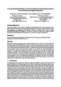
disturbance parameter). Expected tracking performance and very good spectral quality, as confirmed by Fourier analyses shown in Fig. 7(d), (h), are shown for both controllers. Fourier analysis shows the typical spectral behavior of hysteresis controllers operating at variable switching frequency. Switching energy is not concentrated in a narrow region, at multiples of the modulation frequency, but is spread around the average switching frequency. A smoother spectrum results, which is easier to filter out. In Fig. 7(i)–(p), the controllers’ responses to 450-Hz sinusoidal current set points and back EMF are reported (see Table IV, column 2, for disturbance parameters). Good dynamical response under this highly demanding operating condition is shown, joined to a still acceptable spectral quality [Fig. 7(e), (p)]. Very similar current waveforms and spectra are reported for the combinatorial and the sequential controller. Owing to limited occurrence of the type-1) redundancy, where the resolution affects current trajectories, almost the same control vectors are applied to the load in the two cases. The second set of simulation experiments was made to compare different hysteresis controllers in terms of actual transistors’ switching count and frequency, a crucial parameter for the thermal design of the inverter. The results of comparisons are shown in Fig. 8, where the terms switching count and frequency are referred to the sum of commutations (10 to 01 or 01 to 10) in the three legs of the inverter. In the same figure, the average frequency is computed in a time interval of 10 ms, of the same order of magnitude of the typical thermal time constant of power transistors. The proposed controller (both the combinatorial and the sequential implementation) is compared with the hysteresis controllers proposed in [6] and [7], under the same operating conditions and TR amplitude. The controller proposed in [8] is not directly compared, since the reported switching frequency performance is very similar to that in [6]. Suitable equalization actions have been undertaken to ensure congruent results from the controller proposed in [6], defined in a rotating reference frame, and the other controller implemented in a fixed one. Average transistors’ switching frequencies and accumulated switching counts are shown in Fig. 8(a) and (b), while the cumulative frequency distributions (averaged in 10 ms) are shown in Fig. 8(c). The proposed static implementation gives results very similar to those in [7], as expected from conceptually similar (although different in the design approach) controllers. Comparison with the solution in [6] shows that some switching reduction is achieved. The sequential controller has the lowest transistors’ switching frequency (average), joined to a smaller dispersion in frequency values, as clearly shown in Fig. 8(c). A reduction of about 30% with respect to [7] (the best controller among those compared) is shown in the same figure. Comparing the results shown in Figs. 7 and 8, it can be deduced that the main contribution to the switching frequency reduction comes from the type-2) redundancy resolution (zerovoltage vector) that does not affect the current waveforms and spectra reported in Fig. 7.

IV. PROTOTYPE IMPLEMENTATION AND EXPERIMENTAL RESULTS A. Description of the Prototype Controller A prototype board was designed according to the block diagram shown in Fig. 1. A few low-offset operational amplifiers and comparators are used to generate the input patterns for the controller. Logical equations (both combinatorial and sequential) are programmed into an erasable programmable logic device (EPLD). In the adopted prototype, a Lattice ispLSI 1016 EPLD is used. This highly redundant component was adopted in the prototype mainly for its flexibility. Actually, three or four flip-flops and a few combinatorial logical elements are needed for the sequential implementation; an inexpensive GAL can be used. A TEMIC PMC20 integrated /15-A operthree-phase inverter, suitable for 220-V ation, is used in the power section. Current set points are generated by a Rapid Prototyping station developed at the University of Bologna [11]. It must be noted that the increased implementation complexity of the sequential controller with respect to the combinatorial one is negligible. Only three inexpensive flip-flops must be added to the combinatorial logic. B. Disturbances in Hall-Effect Insulated Current Sensors Despite their simplicity, hysteresis controllers need a very careful electronic design. Owing to their very large bandwidth, they are very sensitive to board-generated and measurement noises. The board noise can be controlled by a suitable selection of components and a careful design of the grounding net. Galvanic insulation between the power section and the control part is fundamental to minimize the effects of ground loop noise. To keep insulation between the power side and the control side, an insulated current measurement system has to be used. Insulated current sensors based on the Hall effect are the state-of-the-art current sensors in pulsewidth modulation (PWM)-driven digital current controllers for industrial applications. Owing to the operating principle and constructive characteristics, the most widely used industrial Hall-effect sensors capture an EM-coupled high-frequency disturbance from every transistor switching. This effect is shown in Fig. 9 for some industrial sensors and for the highly sophisticated current probe of a leading oscilloscope manufacturer. Owing to 5- s deadtime in the experimental hardware, the effects of two consecutive switches are present. Although different behaviors characterize the different sensors, the EM disturbance is present in all of them. The sensor, the response of which is shown in Fig. 9(a), is the best performing sensor among all those tested, but still a poorly damped oscillation at about 1 MHz is superposed. Any attempt to reduce noise by signal filtering simply changes the oscillation shape; the amplitude is reduced, but the damping becomes even poorer. The noise superposed to the current measurement can force spurious commutations in large-bandwidth hysteresis controllers. Observation of the disturbance characteristic shows that unfiltered noise has large amplitude, but very short duration. Besides, in


normal operating conditions, the probability of two consecutive commutations is very low. Accordingly, the sequential design of the controller may help to overcome the problem. The simpler solution consists of a synchronous implementation of the finite-state automation. If the sampling period is selected longer than the disturbance transient, the effect of superposed noise is canceled. Unfortunately, an increase of the sampling period leads to some performance degradation, since an equivalent delay is introduced in the loop. An increase of the sampling period deteriorates controller performance, especially when a small TR is adopted. Slightly increasing the complexity of the sequential controller, another solution can be found. A new design is adopted, with a phantom state associated to each state of the Moore model. State transitions always occur toward the phantom state corresponding to the correct one. The system stays in the phantom state (the same control vector as for the corresponding true state is generated) for a programmable number of sampling periods and then goes back to the true state. The scope of these new phantom states is to prevent two consecutive commutations from occurring, owing to the noise transient. The sampling period can be selected again to minimize the delay in the loop. After the noise transient, the normal system operation is recovered, and the next commutation will be generated with the time resolution corresponding to the basic (optimal) sampling period. Since the probability of having two consecutive real commutations is very low, controller performance is almost equivalent to that obtained without sensor noise.

779

(a)

(b)

(c) Fig. 8. Simulation comparison among different controllers. (a) Average frequencies (10 ms). (b) Switching counts. (c) Average-frequency distributions.

C. Experimental Results Owing to the comparable tracking capability and spectral quality of combinatorial and sequential controllers, the latter one was programmed on the EPLD for its better switching properties. The adopted current sensor is the one reported in Fig. 9(a). To overcome the current sensor noise, a synchronous implementation was adopted with 12- s sampling time without using phantom states. During the experimental tests, an IM, the parameters of which are reported in Table V, was used at the inverter load. Two different current set points are applied: 4.2 A /50 Hz (rotating motor) and 1.8 A /450 Hz (locked rotor). In both cases, the amplitude of the TR was selected to be 0.25 and 0.3 A for internal and external regions, respectively. The experimental results, shown in Fig. 10, confirm the very good tracking performance and spectral properties of the proposed controller.

(a)

(b)

(c)

V. CONCLUSIONS A new multivariable hysteresis controller for a three-phase inverter has been proposed in this paper. It is shown that the combinatorial approach to the design of the control logic in multivariable hysteresis controllers currently proposed in the literature has some drawbacks in terms of achievable transistors’ switching frequency. The proposed controller is first presented in its combinatorial implementation, in order to compare performance with those of other controllers proposed in the literature. Then, it is shown how a sequential design

Fig. 9. Output signals for different insulated Hall-effect current sensors after a transistor switching. (a) Standard industrial-type operating at zero field (feedback type). (b) Open-loop-type sensor. (c) Current probe of a leading oscilloscope.

of the control logic can reduce both the transistors’ switching frequency and the frequency spread, with a minimal increase in the complexity of the controller hardware. Controller performance is tested by simulation experiments and compared to that of other similar controllers under the same operating conditions. Simulations confirm good perfor-

780


TABLE V PARAMETERS OF THE TEST IM Parameter Output power Nominal Voltage ( -connected) Nominal Current Poles Stator inductance Rotor inductance Mutual inductance Stator resistance Rotor resistance Rotor inertia

1

Value 1.1 220

Units kW Vrms

4.8 4 0.475 0.475 0.454 6.6 5.5 0.011

Arms Number H H H

Kg1m2

(a)

(b)

(c)

(d)

Fig. 10. Experimental results with the proposed hysteresis (sequential) controller. (a) and (b) Sinusoidal current and spectrum at 50 Hz. (c) and (d) sinusoidal current and spectrum at 450 Hz (locked rotor).

(a)

(b)

(c)

Fig. 11. Interval where the error derivative must be located to ensure stability with the selected control.

error form. Let us consider the eight regions (excluding the TR) where the error can be located by the comparators’ output as shown in Fig. 3(c). Current error converges to the TR in a finite time and remains inside if, starting from an arbitrary initial condition 1) the border of a new region is reached in a finite time; 2) the module of current error component in the direction of the reached border is smaller than the initial one or the error is entered into the TR. Conditions 1) and 2) are ensured if error derivative after application of the selected control voltage is located in a suitable zone, defined according to the error region considered. Three significant situations are shown in Fig. 11: 1) Fig. 11(a), corresponding to one of the four quarter-ofplanes; stability condition is satisfied if error derivative is rotated less than 30 with respect to the control vector; 2) Fig. 11(b), corresponding to one of the two vertical half-strips; stability condition is satisfied if the error derivative is rotated less than 60 with respect to the control vector; 3) Fig. 11(c), corresponding to one of the two horizontal half-strips; stability condition is satisfied if the error derivative is rotated less than 90 with respect to the control vector. Case 1) is the worst case (minimum admissible rotation). Since no a priori information on disturbance orientation is known, the worst disturbance direction must be considered. As can be easily checked by simple trigonometric computations, for each disturbance orientation, the error derivative is rotated less than 30 with respect to the selected control voltage if and only if

mance of both implementations of the proposed controller. It is also shown that the sequential implementation of the proposed controller ensures a 30% reduction of transistors’ switching frequency with respect to the best combinatorial implementation tested. A prototype board implementing the sequential controller has also been presented. In this context, the problem of the EM noise captured by insulated Hall-effect current sensors after each transistor switch is discussed. It is shown how the sequential design can also help in reducing the noise effects. The experimental results obtained with the prototype controller completely confirm the controller performance resulting from simulations.

Condition (A1) ensures a strict convergence to the TR, i.e., once entered, the TR the current error must strictly remain inside. This condition is derived by a worst case analysis. Simulation experiments with typical disturbances have shown that simple stability can also be obtained with a less conservative condition. It must be pointed out that strict convergence condition (A1) depends on the adopted comparators’ topology and the resulting TR shape.

APPENDIX A

APPENDIX B

The stability condition for the proposed controller is derived in a geometrical way, referring to (6) as a system model in

To permit controller evaluation, the Mealy model of the implemented controller is reported in Tables III and IV.

(A1)


TABLE VI STATE–TRANSITION TABLE OF THE IMPLEMENTED SEQUENTIAL CONTROLLER (MEALY MODEL)

Input to Table VI are the sixteen combinations of comparators’ outputs and the eight present states (indicated with capital letters from to ). Output of the table are the future states ( to ) and the associated control vectors ( to ). No residual ambiguities are present in the table and the most suitable control action to ensure system stability and reduced switching frequency is applied in every situation.

781

[4] D. M. Brod and D. W. Novotny, “Current control of VSI-PWM inverters,” IEEE Trans. Ind. Applicat., vol. 21, pp. 562–570, May/June 1985. [5] C. Rossi and A. Tonielli, “Robust current controller for three-phase inverter using finite-state automaton,” IEEE Trans. Ind. Electron., vol. 42, pp. 169–178, Apr. 1995. [6] M. P. Kazmierkowski and W. Sulkowski, “A novel vector control scheme for transistor PWM inverter-fed induction motor drive,” IEEE Trans. Ind. Electron., vol. 38, pp. 41–47, Feb. 1991. [7] C.-T. Pan and T.-Y. Chang, “An improved hysteresis current controller for reducing switching frequency,” IEEE Trans. Power Electron., vol. 9, pp. 97–104, Jan. 1994. [8] J. F. Martins, J. F. Silva, and A. J. Pires, “A novel and simple current controller for three-phase IGBT PWM power inverters—A comparative study,” in Proc. ISIE’97, Guimaraes, Portugal, 1997, pp. 241–246. [9] C. Rossi and A. Tonielli, “Robust control of permanent magnet motors: VSS techniques lead to simple hardware implementations,” IEEE Trans. Ind. Electron., vol. 41, pp. 451–460, Aug. 1994. [10] D. L. Dietmeyer, Logic Design of Digital Systems. Boston, MA: Allyn and Bacon, 1972. [11] R. Morici, C. Rossi, and A. Tonielli, “Fast prototyping of nonlinear controllers for electric motor drives,” in Proc. IFAC World Congr., Sydney, Australia, 1993, pp. 381–386.

Andrea Tilli was born in Bologna, Italy, in 1971. He received the Dr.Ing. degree in electronic engineering in 1996 from the University of Bologna, Bologna, Italy, where he is currently working towards the Ph.D. degree in system science and engineering in the Department of Electronics, Computer and System Sciences. His current interests include nonlinear control techniques, variable-structure systems, electric drives, active power filters, and DSP-based control architectures.

ACKNOWLEDGMENT The authors wish to thank Ing. D. Musiani for his valuable contribution to the initial controller development and to the design of the experimental hardware. REFERENCES [1] R. Marino, S. Peresada, and P. Tomei, “Output feedback control of current-fed induction motors with unknown rotor resistance,” IEEE Trans. Contr. Syst. Technol., vol. 4, pp. 336–347, July 1996. [2] R. Morici, S. Peresada, C. Rossi, and A. Tonielli, “Adaptive output feedback control of current-fed induction motor: A rotating reference frame approach,” in Proc. ECC’95, Rome, Italy, Sept. 1995, pp. 313–318. [3] J. Holtz, “Pulsewidth modulation—A survey,” IEEE Trans. Ind. Electron., vol. 39, pp. 410–420, Oct. 1992.

Alberto Tonielli (A’92) was born in Tossignano, Bologna, Italy, in 1949. He received the Dr.Ing. degree in electronic engineering from the University of Bologna, Bologna, Italy, in 1974. In 1975, he joined the Department of Electronics, Computer and System Sciences (DEIS), University of Bologna, with a grant from the Ministry of Public Instruction. In 1979, he started teaching as an Assistant Professor. In 1980, he became a Permanent Researcher. Since 1985, he has been an Associate Professor of Control System Technologies. In 1981, he spent two quarters at the University of Florida, Gainesville, as a Visiting Associate Professor. His current research interests are in the fields of nonlinear and sliding-mode control for electric motors, nonlinear observers, robotics, and DSP-based control architectures.