The first application of nuclear magnetic resonance spectroscopy (NMR, ... Those
books on biological NMR, while still very useful, tend to be somewhat.
1 Introduction
The first application of nuclear magnetic resonance spectroscopy (NMR, sometimes referred to as n.m.r. in old-fashioned texts) to a biological sample was reported1in 1954 by Jacobson, Anderson, and Arnold on the effect of hydration of deoxyribonucleic acid, one year after Watson and Crick's historic discovery. Three years later, Saunders, Wishnia, and Kirkwood obtained the first 'H NMR spectrum of a protein, ribon~clease.~ This spectrum, obtained at 40 MHz, is shown in Fig. 1.1. In contrast, the 750 MHz 'H NMR spectrum of the enzyme lysozyme is shown in Fig. 1.2. In the intervening 38 years, the field of NMR spectroscopy has undergone a revolution, culminating in the award of the 1991 Nobel Prize for Chemistry to Richard Ernst, one of the key figures in the development of NMR. However, the recognition given to this field is only just beginning, and the area where the method is likely to have the greatest impact is at the interface between biology, chemistry, and physics. Although there are a number of excellent texts on NMR spectroscopy, they are primarily for chemists, and tend'to focus either on the theory of NMRM or on applications to organic chemistry. Those books on biological NMR, while still very useful, tend to be somewhat outdatedg-l2or directed solely towards structure.13This book seeks to provide a general outline of basic NMR theory and examine selected examples of applications to
197
0
Cycles.
Fig. 1.1 The first 'H NMR spectrum of an enzyme, ribonuclease, at 40 MHz, obtained in 1957. (Reprinted from Ref. 2 with permission.)
5
Basic theory of N M R
dimensional structures of individual components in the cell, such as proteins, enzymes, DNA, RNA, and membranes. Therefore, a technique which can obtain an image of a human head on the one hand, and the structure of DNA on the other, must be worth learning about. The following sections will attempt to provide sufficient basic NMR theory for use in solving biological problems. Throughout this book the emphasis will be on molecular details rather than macroscopic details such as the images obtained with MRI. There are a number of excellent texts on the MRI technique, and the reader is referred to those for more information.14-l5
1.1 BASICTHEORY OF N M R This chapter attempts to provide a brief summary of the salient features of basic NMR theory. It does not presume to be exhaustive, and the reader should refer to one or more of the increasing number of texts in this area for more detailed information (vide supra). In our treatment of NMR theory we have chosen to introduce both classical vector formalism and also quantum mechanical Cartesian product operator formalism. In our experience vector formalism, while being extremely useful for simple experiments, is not very helpful in understanding multidimensional NMR experiments. Rather than introduce the far more complicated density operator formalism, we make no apology for adopting the produce operator formalism where appropriate. The mathematics follows simple rules, and, while sometimes generating lengthy expressions, algorithms are even for computer programs such as Mathematica. The product operator formalism is relatively straightforward and very powerful, and is now the method of choice for evaluating new pulse sequences. It is important for researchers using NMR to be familiar with it.
1 .I .I The N M R phenomenon The magnetic resonance phenomenon occurs as a result of the quantum mechanical property of spin. This is a source of angular momentum intrinsic to a number of different nuclei. The spin angular momentum confers a magnetic moment on a nucleus and therefore a given energy in a magnetic field. The nuclear spin (I) can have the values I = 0, 21, 1, l;, . . . ,etc. (see Table 1.1). Note that common biological nuclei such as 12Cor 160have I = 0 and therefore do not give NMR spectra. The nuclear magnetic moment ( p ) is given by:
The gyromagnetic ratio (also known as the magnetogyric ratio) y is the proportionality constant which determines the resonant frequency of the nucleus for a given external field. Typical nuclei of interest in biological NMR are given in Table 1.2. In a magnetic field, a nucleus of spin I has 21 1 possible orientations, given by the value of the magnetic quantum number m,, which has values of - I, - i + 1, . . . I - 1 (e.g. for a nucleus of spin i, m -- - 2 i, $).We can regard a spin-; nucleus as a small bar magnet, which when placed in a static field has an energy which varies with orientation to the field. The possible energies are quantized, with the two possible values of m,(+;) corresponding to parallel and antiparallel orientations of this small magnet and the external field. As we shall see
+
,,-4,
6
Introduction
Table 1.1 Mass no.
Atomic no.
I
Odd
Even or odd Even
0
Odd
1,2,3 . . .
Even Even
1 3 5 2, 2,
...
shortly, the NMR absorption is a consequence of transitions between the energy levels stimulated by applied radiofrequency (RF) radiation. Although we should bear in mind the quantized nature of nuclear spin, we can describe the motion of a nucleus in a magnetic field in terms of classical mechanics. In the presence of an applied magnetic field B,, the magnetic moment experiences a torque which is the , (see vector product of the nuclear angular momentum J and the magnetic moment u Fig. 1.3). Note, however, that the physical picture presented here does not represent reality. The findings of the famous Stern-Gerlach experiment clearly suggest that spin angular momentum is quantized, and therefore classical mechanics is not applicable. Furthermore, the nucleus is not necessarily spinning about its axis-indeed were it to be spinning the radial velocity would exceed the speed of light. Thus although we speak of 'spin' as if the nucleus were actually rotating about its axis, this is an unfortunate choice of words since the source of the magnetic moment is a purely quantum mechanical property which could just as easily be called 'sweetness', 'bitterness', or whatever. According to Newtonian mechanics, this torque equals the rate of change of angular momentum :
Fig. 1.3 Schematic representation of the motion of a nucleus in a magnetic field.
Table 1.2 Magnetic properties of some biologically useful nuclei Isotope
Spin
Natural abundance (%)
Quadrupole moment Q (1 0-28 m2)
Gyromagnetic ratio y (1 O7 rad s-' T-')
"At constant field for equal number of nuclei. bProduct of relative sensitivity and natural abundance.
Sensitivity re1.a
ab~.~
NMRfrequency (MHz) at a field tT) of 2.3488
8
Introduction
'
2 = y p x ~ ousing p = y ~ h = y ~ dt
(1.4)
This equation is analogous to the equation of motion for a body with angular momentum L in a gravitational field g with mass m at a distance r from the fixed point of rotation, if we equate J to L and B, to g,and regard r x m as an intrinsic property of the body analogous to YP :
Thus this is just like the motion of a gyroscope which in a gravitational field precesses, i.e. its axis of rotation itself rotates about the field direction. In the classical analogy, the same motion occurs for nuclear spins in a magnetic field. The energy of the interaction is proportional to p and B, (see Fig. 1.4), so
and since Am, = 1,
AE = yhBo and from Planck's law,
AE= hv then V =yBO - (in HZ)
27t
or co=yB, (in rad s-') Note that we have dropped the minus sign between Equations (1.6) and (1.7). This is a convention that has been widely adopted for convenience in the NMR literature, although, as pointed out by Ernst and co- worker^,^ strictly speaking, o = - yB,, which
Fig. 1.4 Energy level diagram.
Basic theory of N M R
9
has consequences for the Cartesian representation of vectors and product operators considered in Sections 1.1.2 and 1.1.3. Thus nuclei precess around the B, axis at a speed which is called the Larmor frequency (which is its NMR absorption frequency, o).The rotation may be clockwise or anticlockwise depending on the sign of y, but is always the same for any particular nucleus. The two energy states a and P will be unequally populated, the ratio being given by the Boltzmann equation:
Another way to look at this is that in a sample containing a large number of spins, all possessing the same Larrnor frequency, the parallel orientation of the z component of each spin along the B, direction is of lower energy than the antiparallel one. So at thermal equilibrium, we expect the Boltzmann surplus as shown in Fig, 1.5. Thus along the z axis there is a net magnetization of the sample parallel to the field. All the contributing spins have components precessing in the xy plane, but because all have equal energy, the phase of the precession is random. Thus for an ensemble of spins, there is no net magnetization in the xy plane and total magnetization of the sample is stationary and aligned with the z axis (called M,).
1 .I .2 The vector model Radio frequency (RF) radiation is electromagnetic (see Fig. 1.6) and can be represented as an oscillating magnetic field, which in turn can be represented by magnetization vectors (see Fig. 1.7). This represents the half cycle of the oscillation of the magnetization due to the presence of the R F (also known as the B,) field. Alternatively, we can represent its as two magnetization vectors of constant amplitude rotating about an axis (x) in opposite directions, with angular frequency = RF. Thus phis pair of counter-rotating vectors is a valid way of representing the R F (see Fig. 1.8). So when the sample and the R F field interact, we have a moving field interacting with a static one (although this, too, causes precessional motion in the sample). Conceptually, the way this rather complex picture is simplified is by rotating the coordinate axes at the same rate as the nuclear precession. Now since there is no precession, it looks as though the applied field (which caused the precession) has disappeared. However, the net magnetization remains along the z axis. Furthermore, the RF can be decomposed into two
+
(static field)
(static field)
z
(bulk magnetization vector) Y
Fig. 1.5 The bulk magnetization vector.
components, one in the xy plane. The other, which was originally moving at an equal speed in the opposite direction, is rotating in the new frame at twice the Larmor frequency. This can now be neglected, and has no effect on the NMR experiment (see Fig. 1.9). When a pulse of RF is applied to the sample, i.e. the B, field is switched on and then switched off, in the rotating frame the M, and B, vectors are static and orthogonal. This generates a torque and the sample magnetization is driven around by the B,vector, at a speed dependent on the field strength. Thus we could move it through 90°, as shown in Fig. 1.10. Note that the direction of motion (in this case clockwise relative to the B, direction) is to some extent arbitrary, and in general the NMR literature using classical vector formalism adopts the convention used here (although the opposite convention has
Fig. 1.6 Electromagnetic nature of RF radiation with oscillating magnetic and electric fields.
Fig. 1.7 RF radiation represented by magnetization vectors.
Fig. 1.8
RF radiation represented by two counter rotating vectors.
'
RF vectors
LABORATORY FRAME
ROTATING FRAYE
Fig. 1.9 Magnetization vectors shown in the laboratory and rotating frames.
11
Basic theory of N M R
been adopted when using the Cartesian representation of product operators-see Section 1.1.3). Note, however, that the direction is governed by the sign of the gyromagnetic ratio. After the pulse has finished, the sample magnetization remains in the xy plane. In the laboratory frame it precesses about the static field, generating radio signals (see Fig. 1.11). These radio signals generate what is called the free induction decay (FID), which is a function that decays exponentially with time (see Fig. 1.12). The F I D is related to the frequency domain spectrum through Fourier transformation. This is as follows :
lz :1
Re(f(co)) =
-
f (t)cos cot dt
-/.
Im(f (co)) =
f(t)sin cot dt
since eK"=cos ot + i sin ot (see Fig. 1.13). This is a consequence of the fact that every NMR signal has amplitude, frequency, and phase. The NMR signal is detected using a
on off
RF off
Fig. 1.10 The sample magnetization driven to t h e y axis after a 90' pulse.
Ty/ Static
on RF off
(wx
ROTATING FRAME
.--..-.----
I
Precessing about B,
After time t
off
LABORATORY FRAME
Fig. 1 .I 1 Precession of the sample magnetization about the static field.
12
Introduction
t
Fig. 1.1 2 The free induction decay.
Pure ~ b d o r ~ t i oLineshape n
Pure Dispersion Lineshape
Fig. 1.1 3 Pure absorption lineshape versus pure dispersion lineshape.
Magnet
- Sample
COMPUTER
w Transmitter
Fig. 1.1 4 Outline of a NMR spectrometer.
13
Basic theory of N M R
detector, and the basic outline of an NMR spectrometer is given in Fig. 1.14. This represents a greatly simplified picture of a modem NMR spectrometer, which nowadays is commonly equipped with three RF channels and an array of sophisticated equipment, a discussion of which is outside the scope of this book. However, one feature which is particularly important is the way in which the signal is detected. Here a technique known as quadrature detection is used. The detectable magnetization can be represented as a vector precessing in the xy plane, as we saw in Fig. 1.9, so that a detector aligned along the x axis would be insensitive to the direction of rotation of the vector. In other words, the detector cannot distinguish whether the signal frequency is greater or less than the reference frequency in the case where two signals are on opposite sides of the reference by the same frequency difference. The two vectors would be rotating at the same frequency but in opposite directions. In order to distinguish between these we use a detector that can detect the signals along both they and x axes simultaneously. Instead of having two coils, however, the signal is manipulated electronically, by having two detectors in which one has had the phase of the reference frequency shifted by 90" and the FIDs stored in separate memory locations in the computer. Since the phase of one of these FIDs is affected by the sign of the frequency, these two FIDs correspond to the real and imaginary components of the signal, and are treated as such in the Fourier transformation. The question of phase both in terms of the transmitter pulses and in terms of the receiver is important. In many pulse sequences, as we shall see later in this chapter and in Chapter 2, elaborate phase cycling of pulses and the receiver are required in order to achieve the particular result desired. This is the means by which desired and undesired signals are separated. The same result can also be achieved using what are called pulsed jield gradients, which are emerging as an important and fast alternative to lengthy phase cycles.'* An example of the consequence of changing the phase of the transmitter pulses is summarized in Fig. 1.15, which uses the vector model to represent the four possible phases ( x , y, - x, and -y).
90°, pulse
Y
Fig. 1.I 5 T h e vector representation of R F pulses of differing phase.
14
Introduction
1.I .3 The product operator There are intrinsic limitations in representing the effects of R F pulses in NMR using vectors, and we need to consider alternative ways of looking at this. In contrast to the vector formalism, in which the macroscopic magnetization rotates under the influences of pulses, and/or precesses under the influence of chemical shift, the entire state of the spins or spin system can be described by the wave function, Y(t), or the density operator a(t). Disregarding relaxation, the time evolution of the density operator is described by the Liouville-von Neurnam equation:
Z ( t ) is the famous Harniltonian operator, which includes chemical shift terms, coupling terms, and so on. Instead of getting into the rather complex area of density matrices, we can describe the density operator in terms of Cartesian product operators.lg Thus the ground state of a system at thermal equilibrium is described by a polarization (or population-see Section 1.1.7) along the z axis, I,. After a pulse in the y direction:
I,
I,
(XIY
aIy
I, cos a - I, sin a
(1.15)
+
(1.17)
I, cos a I, sin a
These Cartesian operators, I,, I,, and I, transform like magnetizations when a rotation is performed. The properties of a state I,, I,, and I, can be read off directly with such simple operators, since they each consist of only one operator. I, is associated with an x magnetization, and I, and I, accordingly. We will adopt the following convention: aI,, or ale = flip angle a about an axis in the xy plane (forming an angle with the x axis)
4
SZI,t = evolution of chemical shift SZ of nucleus I during time t 271J11,12,t=ev~lutionof coupling J between nuclei I, (or I) and I, (or S) during time t So for chemical shifts:
I,
I,,
ad,
nt1,
+
I, cos fit 1, sin Qt I, cos fit - I, sin SZt
Basic theory of N M R
15
Detection of x magnetization leads to build-up of the signal according to the coefficient -sin Qt of I,. Fourier transformation leads to a line at $2.Quadrature detection allows selection at either SZ or -Q . Thus we can summarize the vector model and the product operator model as in Fig. 1.16 for a simple 90" pulse. The effects of chemical shifts, pulses, and positive scalar couplings on product operators are summarized pictorially in Fig. 1.17, and summarized mathematically in Appendix 1. Note that the sense of rotation for product operators is opposite to the classical description presented in Section 1.1.2. As
+
+
on
z3
Detection
I
I
Fourier
\
UV'-
L-
transformation
C--
o
I 9O0y p u l s g Ix
,+
Evolution
during detection
Ixco~t IysinRt
Spectrum
Vector representation for the magnetization of a nucleus without coupling
Corresponding product operators for one kind of nucleus
Fig. 1.16 The vector model and the product operator model for a 90" pulse.
Coupling
Fig. 1 .I7 Graphic representation of the effect of chemical shifts, pulses, and positive scalar couplings on product operators. (Reprinted from Ref. 4 with permission.)
16
Introduction
mentioned in Section 1.1.1, this results from the fact that, strictly speaking, co = - yB,, and when product operator formalism was introduced, the minus sign was retained, thereby changing the sense of the rotation relative to classical formalism. Of course this has nothing to do with the physics, and is simply a consequence of how the equations are written.
1 .I .4 Relaxation Having considered how we obtain xy magnetization, let us turn to what happens to it after the R F pulse is switched off. Naturally, it might be expected to return eventually to thermal equilibrium along the z axis. The time it takes to do this is relatively long compared to other spectroscopic techniques, and constitutes an important aspect of the experiment. In the Bloch theory of relaxation, the assumption is made that equilibrium will be approached exponentially. Thus magnetization will build up (or decay) according to:
Longitudinal relaxation ( T,) The build-up of M, can be represented as shown in Fig. 1.18. Thus if M, is the magnetization at thermal equilibrium, then M, = Mo(l - e-'ITl)
T , is called the longitudinal (or spin-lattice) relaxation. After a
pulse, the magnetization precesses about the z axis in the xy plane. With longitudinal relaxation, the
t
Fig. 1.1 8 Build-up of magnetization (MJ.
7112
17
Basic theory of N M R
z magnetization reappears (see Fig. 1.19) with the time constant TI.One common method
for the measurement of T,s is the inversion-recovery method, which is shown in Fig. 1.20.
Transverse relaxation ( T2) The transverse relaxation, or T2,is not intuitively obvious, and is harder to understand in simple physical terms. When the magnetization is in the xy plane, there is phase coherence between the spins in the transverse plane, and loss of this phase coherence due to mutual exchange of spin energies is what gives rise to T2 relaxation. However, in general, T2 is always greater than T,, and this is because there are additional causes of loss of transverse magnetization. Disregarding longitudinal relaxation (T,) for a moment, the static magnetization in the xy-plane would not remain there because of another simple fact: the static field is not uniform throughout the sample. Thus, if we divide up the sample into small regions such that the field is uniform (regions known as isochromats), then the total magnetization is the sum of all these regions, each of which contributes a precessing vector which differs slightly in frequency. This blurs the bulk magnetization vector, and this is due to inhomogeneous broadening, which often dominates the transverse (or spin-spin) relaxation, T2. Note that the magnetic field inhomogeneity is really an experimental artefact, and when it dominates T, the directly observed decay is usually defined as T,* whereas T, is usually reserved for other causes of loss of order (see Fig. 1.21).
Spin echoes One of the fascinating things that happens if we apply two RF pulses in quick succession relative to TI is the production of a spin echo. Consider the pulse sequence (7~12)- z - n shown in Fig. 1.22. After the n/2 pulse, the inhomogeneity causes the isochromats to fan
Fig. 1.19 Reappearance of the z-magnetization.
XX
t
Fig. 1.20 The inversion recovery method.
(WX
Acquire
18
Introduction
out. The front edge is labelled ' + ' for the vectors precessing faster than a,,and the back edge is labelled '-' for the slower vectors. The n, pulse rotates all the isochromats together about the x axis, leaving the vectors on they axis. Now the ' + ' sign lags behind the average direction of the vectors and the ' - ' side is ahead. Thus the faster vectors catch up with the average position and the slow ones fall back to it. Thus after an additional time they refocus to give an echo. In fact, in a sense, time has been reversed, since the disorder in the system can be rever~ed.~' Let us also consider the product operator calculation for this pulse sequence: a, = I, 5.9% a,= -Iy
1nr4 a,= -Iy cos Rr+Zx sin SZz
1 180,
a,= -Iy cos Rz- I, sin SZr
1 QzZz
a, = -Iy cos2Rr + I x cos Rr - sin Rz - Zz cos
. sin Rr - I,, sin2Rz
I
i
M, isochromats
f
resultant My
Fig. 1.21 The vector model of transverse relaxation (T,).
(d2h
Fig. 1.22 The spin echo method.
t/2
XX
ff2
-Acquire
Basic theory of N M R
19
So note that we have essentially returned to where we started after the first 90" pulse. Remembering this point greatly simplifies product operator calculations, since many pulse sequences use spin echo sequences to refocus chemical shifts. Spin echoes play a very important role in modern NMR experiments. For example, two lines of different chemical shifts evolve at different rates in the rotating frame, so if we apply an echo sequence, they diverge before the 180" pulse, but realign after it. Similarly, heteronuclear couplings are refocused by spin echoes, but not homonuclear couplings. Spin echoes can be used to measure q s , although there are inherent difficulties in such measurements. An alternative method is to simply measure the linewidth, since v,,, = 1/nq ,where vl12 is the linewidth at half-height. Another spin echo sequence, and the one usually used in practice, is the Carr-PurcellMeiboom-Gill spin echo sequence, which is:
Cumulative errors due to an incorrectly set pulse length do not arise. We can illustrate this if we consider the fate of the fastest moving isochromat only and look at the consequence of the pulse angle being not TC but some slightly different value TC -E, as shown in Fig. 1.23. Consider a pulse 13= TC - E, which is slightly shorter than TC and directed along they axis. The pulse interchanges the orders of rotation of the slow and fast magnetization isochromats (Fig. 1.23(c)), and leaves them slightly above the xy plane. Refocusing then occurs normally at time 22 but takes place above they axis in the zy plane (Fig. 1.23(d)). After the dephasing period 2 (Fig. 1.23(e))the second TC- E pulse rotates the isochromats
(a) rJ2 pulse
Fig. 1.23 Vectorial representation of the Carr-Purcell-Meiboom-Gill spin echo.
20
Introduction
exactly back into the xy plane where they are refocused at time 42 (Fig. 1.23(g)). Thus all the even-numbered echoes are produced along the right direction,^, whereas all the oddnumbered echoes are only slightly displaced and by a constant angle.
1 . I .5 The nuclear Overhauser effect The Nuclear Overhauser Effect (NOE, q ) is the change in the intensity of an NMR resonance when the transitions of another are perturbed. Generally, this means saturation, which is the elimination of a population difference across some transitions (by irradiating one with a weak RF field) while observing the signals from others: where I, is the thermal equilibrium intensity. Consider two spin-i nuclei I and S, with the same y but different chemical shifts and not J coupled where the energy levels are represented as combinations of a and P, and the populations indicated with multiples of N. The system is shown in Fig. 1.24. Chemical shifts are very small compared with the Larmor frequency (i.e. of the order of ppm), so the transitions have nearly equal energy. Assuming we have 4N nuclei, then each energy level would have N nuclei of almost equal energy. The population differences are given in Table 1.3. The first four differences in Table 1.3 are across the normal transitions which give rise to the NMR lines, while the other two involve changes in the quantum number M (which is the total of the individual quantum numbers m for the two nuclei). Although these latter two are not observable, they may contribute to the relaxation pathways. Another way of looking at this is to consider how the system restores itself. The relaxation can take place in several ways and we can assume that relaxation across a single transition is first order, and the rate constant is designated W, with the subscript distinguishing the change in M involved (see Fig. 1.25). TIis therefore related to some combination of W:, W2,and Wo. If W2 and Wo= 0, then
Note that if W2and Wo# 0 then the total relaxation time for spin I involves transitions of spin S. Thus T, measurements on multispin systems are not straightforward.
/-"
Saturated
Populations and energy levels of a homonuclear AX svstem
Populations of the levels immediately following saturation of the S transitions
Fig. 1.24 Populations of levels before and after saturation of the S transitions.
Basic theory of N M R
Table 1.3 Population differences for transitions between energy levels in onedimensional NOE experiment At thermal equilibrium
I transitions: S transitions:
h = O transition: Am= 2 transition:
Pa-PP aB-PB Pa-aa aa-/3/3
After saturation of S
) )0 26
If only single-quantum transitions were involved, saturation of spin S would result in no change in intensity for spin I. It is the so-called zero- and double-quantum transitions, Wo and W2that enable us to detect the NOE. If Wo is the dominant relaxation pathway, saturating S decreases the intensity of the I resonance, and there is a negative NOE at I due to S. Conversely, if W2is the dominant relaxation pathway, saturating S increases the intensity of the I resonance, and there is a positive NOE at I due to S. The steady-state NOE enhancement at spin I on saturation of spin S is described by the Solomon equation :21
Deriving Equation (1.27) is outside the scope of this book, but interested readers should refer to the book by Neuhaus and Williarn~on.~~ Note that for homonuclear NOEs y,= y, and typically the maximum enhancement is ~ 5 per 0 cent whereas for heteronuclear NOEs the enhancement is also multiplied by the ratio of the two ys.
Mechanisms for relaxation The interaction which gives rise to the NOE is the dipolar coupling between nuclei. This is the interaction between nuclear magnetic dipoles, in which the local field at one nucleus is due to the presence of the other. Since this local field is dependent upon the orientation of the whole molecule, it may vary from one molecule to the next. In amorphous or
Relaxation pathways immediately following saturation of the S transitions
Fig. 1.25 Relaxation pathways before and after saturation of the S transitions.
22
Introduction
polycrystalline solids, where the positions of single molecules are fixed, but vary from one molecule to the next, this leads to a range of resonant frequencies and characteristically broad lineshapes. In single crystals, the lineshape is dependent upon the orientation of the crystal with respect to the magnetic field. In solution, rapid molecular motion averages the dipolar interaction, generating fluctuating fields which stimulate longitudinal relaxation. The strength of the dipolar interaction is dependent upon internuclear distance, and can cause the cross-relaxation that gives rise to the NOE.
1 .I .6 Dipolar coupling The relation between dipolar coupling, TI and NOE is connected through z,, the rotational correlation time. Since the size of the dipolar interaction does not depend on z,, but its rate of change does, the total power available from the lattice will be constant (i.e. the area underneath the curve of spectral density versus frequency-see Fig. 1.26), while the upper limit of their frequencies will vary with 2,. Thus if the strength of the fluctuating field, the spectral density function J(o), is plotted against frequency, equal areas are enclosed, but the upper limits vary (see Fig. 1.26). The spectral density is simply the Fourier transform of a correlation functiong(t), and a correlation function establishes a correlation between a parameter at time t and at some time later (t z), for example it correlates the isotropic motion of a molecule with time, and its rate constant for the decay is in fact the rotational correlation time, 2,. We are assuming that the spectral density is constant for co4 l/z,. This then allows predictions to be made about the variation of TI, T2and Ws with z,. For example, as z, decreases, o, also decreases, and therefore TI increases. At l / z , ~ o ,there is a point of inflexion. What is found is shown in Fig. 1.27. For W,, W, and W2 relaxation we would predict that in this region at the point of inflexion W, would fall off first since it is the sum of two transitions. Without deriving them, the quantitative relaxation rates via dipolar coupling are :
+
W:
K
32c
r6(1+LC);Z:
+
cc 32 r
wo ~c r6(1+ ( a3% I-
(under extreme narrowing)
2:)
122,
w2cc r6(1+ + US)
2
(01
22 r6
K --"
122,
2
2,)
K~
(under extreme narrowing)
(under extreme narrowing)
(1.30)
Assuming 1/z, o, might also be expressed as oiz: < 1, which is called the extreme narrowing limit, then the terms above simplify as shown, with the famous 1/r6dependence for NOE. Note, therefore, that for biological macromolecules, this extreme narrowing limit does not hold, and interpretation of the l / r 6dependence is not straightforward. Although the dipolar interaction, modulated by molecular motion, is the most important relaxation mechanism in solution for protons and other spin-; nuclei such as 13C, there are other mechanisms which should be mentioned. Indeed, the overall T, is
Basic theory of NMR
23
comprised of many contributing relaxation mechanisms:
T;'= T-1 + T-1 + 7'-'+ T-1 + T-1 IDD ~ S R IQ ISC ICSA
(1.31) In addition to dipolar (TiDD)relaxation, there is paramagnetic relaxation, which is a dipolar interaction with the very large magnetic moment of an unpaired electron; and spin-rotation (Ti,) in which there is segmental motion of an aromatic ring, for example. Also, there is quadrupolar relaxation (T,& which is due to the coupling of electric field gradients with nuclei possessing a quadrupole moment, scalar coupling relaxation (TI,,),
P)
Fig. 1.26 Plot of the spectral density function J(o)against frequency (o).
-1 2
-10
-8
-6
-4
Log1o(% Is)
Fig. 1.27 Variations of
T,and T,as a function of r,.
-2
24
Introduction
which is due to rapidly changing coupling networks; and finally chemical shift anisotropy (T,,,,), which is due to modulation of the chemical shift tensors (a,, ,a,, ,and a,,) due to molecular motion. The 'H{'H) NOE, which is of prime interest for conformational studies, is 0.5 for the extreme motional narrowing situation (wiz:< 1, or zC