Fuzzy unconstrained Parametric Geometric

Journal of Fuzzy Set Valued Analysis 2016 No. 2 (2016) 125-139 Available online at www.ispacs.com/jfsva Volume 2016, Issue 2, Year 2016 Article ID jfsva-00301, 15 Pages doi:10.5899/2016/jfsva-00301 Research Article

Fuzzy unconstrained Parametric Geometric programming problem and its application Wasim Akram Mandal1*, Sahidul Islam2 (1) Beldanga D.H.Sr.Madrasah, Beldanga-742189, Murshidabad, W.B, India (2) Department of mathematics, University of kalyani, kalyani, W.B, India

Copyright 2016 © Wasim Akram Mandal and Sahidul Islam. This is an open access article distributed under the Creative Commons Attribution License, which permits unrestricted use, distribution, and reproduction in any medium, provided the original work is properly cited.

Abstract In this paper, we have proposed fuzzy unconstrained geometric programming (GP) problem and modified geometric programming (MGP) problem with negative or positive integral degree of difficulty. Geometric programming technique provides a powerful tool for solving optimization problems. Here we use nearest interval approximation method to convert a triangular fuzzy number to an interval number. In this paper, we transform this interval number to a parametric interval-valued functional form and then solve the parametric problem by geometric programming technique. Here some necessary theorems have been derived. Finally, these are illustrated by numerical examples and applications. Keywords: Unconstrained problem, Modified fuzzy Geometric programming problem, Fuzzy numbers, Intervalvalued function. 2010 Mathematics Subject Classification: 90B05, 90C70.

1 Introduction Since late 1960’s, Geometric Programming (GP) used in various field (like OR, Engineering science etc.). Geometric Programming (GP) is one of the effective methods to solve a particular type of Non linear programming problem. The theory of Geometric Programming (GP) first emerged in 1961 by Duffin and Zener. The first publication on GP was published by Duffin and Zener on (1967). There are many references on applications and methods of GP in the survey paper by Ecker. They describe GP with positive or zero degree of difficulty. But there may be some problems on GP with negative degree of difficulty. Sinha, et al., proposed it theoretically. Abot-El-Ata and his group applied modified form of GP in inventory models. S. Islam, T.K. Roy [17] (2006) presented modified geometric programming (MGP) and its applications, they also presented Multi-Objective Geometric-Programming Problem and its Application.

* Corresponding Author. Email address: [email protected]; Tel: +91 9153222799 125

Journal of Fuzzy Set Valued Analysis 2016 No. 2 (2016) 125-139 http://www.ispacs.com/journals/jfsva/2016/jfsva-00301/

126

In 1990 R.K.Varma has studied fuzzy programming technique to solve geometric programming problem. Biswal (1992) developed fuzzy programming with non linear membership functions approach to multiobjective GP problems. Cao[2] (1992), is the first one to transform Geometric programming problem (GP) to its corresponding fuzzy state and has shown that Fuzzy programming is an useful method to solve multiobjective optimization problem. In this filed a paper named geometric programming problem with fuzzy parameters and its application to crane load sway by S. Yousuf, N. Badra and T.G Abu-El Yazied has been published in world applied science journal in 2009. Bit developed fuzzy programming with hyperbolic member functions to solve GP with several objective functions. A solution method of posynomial geometric programming with interval exponents and coefficients was developed by Liu [12] (2008). Kotba, Halla, Fergancy[8] (2011), presented Multi-item EOQ model with both demand depended unit cost and varying Lead time via Geometric Programming. Samir Dey and Tapan Kumar Roy [14] (2015) presented Optimum shape design of structural model with imprecise coefficient by parametric geometric programming. In this paper we have proposed fuzzy unconstrained GP and MGP problem with negative or positive integral degree of difficulty. Here we transform interval number to parametric interval-valued functional form and then fuzzy geometric programming problem becomes fuzzy parametric geometric programming problem, for that purpose some necessary theorems have been derived. Finally, these are illustrated by numerical examples and applications. 2 Fuzzy number and its nearest interval approximation: 2.1. Fuzzy number A real number 𝐴̃ described as fuzzy subset on the real line ℛ whose membership function 𝜇𝐴̃ (𝑥) has the following characteristics with −∝< 𝑎1 ≤ 𝑎2 ≤ 𝑎3 0, 𝜕𝐶 2 (D(𝐶𝐿 ∗, 𝐶𝑅 ∗)) =2 > 0 and 𝐿 𝑅 𝜕2 𝜕2 𝜕2 ∗ ∗ ∗ ∗ H(𝐶𝐿 , 𝐶𝑅 ) = 𝜕𝐶 2 (D(𝐶𝐿 , 𝐶𝑅 )). 𝜕𝐶 2 (D(𝐶𝐿 ∗, 𝐶𝑅 ∗)) – (𝜕𝐶 ∗ 𝐶 ∗ (D(𝐶𝐿 ∗ , 𝐶𝑅 ∗ )) )2 = 4 > 0. 𝐿 𝑅 𝐿 𝑅 So D(𝐶𝐿 ∗, 𝐶𝑅 ∗) i.e. d(𝐴̃, 𝐶𝐷 (𝐴̃)) is global minimum. Therefore, the interval 1 1 Cd(𝐴̃) = [∫0 𝐴𝐿 (𝛼)𝑑𝛼, ∫0 𝐴𝑅 (𝛼)𝑑𝛼] is the nearest interval approximation of fuzzy number

𝐴̃ with respect

to the metric d. Let 𝐴̃ = (a1, a2, a3) be a triangular fuzzy number. The α-cut interval of 𝐴̃ is defined as Aα = [AL (α), AR (α)] where AL (α) = a1+α(a2 - a1) and AR (α) = a3 - α(a3 – a2). By nearest interval approximation method the lower limit of the interval is 1

1

a1 +a2 and the upper limit of the 2 1 1 a3 +a2 CR = ∫0 𝐴𝑅 (𝛼)𝑑𝛼 = ∫0 [a3 − α(a3 − a2 )]dα = 2 . a +a a +a Therefore, the interval number corresponding 𝐴̃ is [ 1 2 2 , 3 2 2 ] = [𝑚, 𝑛]. In 1 1 form the interval number of ̃𝐴 is defined as 〈4 (a1 + 2a2 + a3 ), 4 (a3 −a1 )〉.

CL = ∫0 𝐴𝐿 (𝛼)𝑑𝛼 = ∫0 [a1 + α(a2 − a1 )]dα =

interval is

the centre and half –width

2.4. Parametric Interval-valued function Let [m, n] be an interval, where m > 0, n > 0. From analytical geometry point of view, any real number can be represented on a line. Similarly, we can express an interval by a function. The parametric interval-valued function for the interval [m, n] can be taken as g(s) = 𝑚1−𝑠 𝑛 𝑠 for s ∈ [0,1], which is a strictly monotone, continuous function and its inverse exits. Let 𝜓 be the inverse of g(s), then s=

𝑙𝑜𝑔𝜓−𝑙𝑜𝑔𝑚 . 𝑙𝑜𝑔𝑛−𝑙𝑜𝑔𝑚

3 Unconstrained problem 3.1. Geometric Programming problem with fuzzy coefficient: Primal fuzzy geometric programming problem is of the form 𝑇0 𝛼0𝑘𝑗 Min 𝑔̃0 (x) = ∑𝑘=1 𝑐̃𝑜𝑘 ∏𝑚 𝑗=1 𝑥𝑗 Subject to

(3.1)

𝑥𝑗 >0,

International Scientific Publications and Consulting Services


128

Here 𝛼0𝑘𝑗 are real numbers and coefficients 𝑐̃0𝑘 are fuzzy triangular numbers, as 𝑐̃0𝑘 = (𝑐1 0𝑘 , 𝑐 2 0𝑘 , 𝑐 3 0𝑘 ). Using nearest interval approximation method, we transform all triangular fuzzy number into interval number i.e. [𝑐0𝑘 𝐿 , 𝑐0𝑘 𝑈 ].The geometric programming problem with imprecise parameters is of the following form 𝑇

𝛼0𝑘𝑗 0 Min 𝑔̂0 (x) = ∑𝑘=1 𝑐̂0𝑘 ∏𝑚 𝑗=1 𝑥𝑗 subject to 𝑥𝑗 > 0,

(3.2)

Where 𝑐̂𝑜𝑘 𝑑enotes the interval counter parts i.e., 𝑐̂0𝑘 ∈ [𝑐0𝑘 𝐿 , 𝑐0𝑘 𝑈 ]. 𝑐0𝑘 𝐿 > 0, 𝑐0𝑘 𝑈 > 0, for all k. Using parametric interval-valued functional form, the problem (3.2) reduces to 𝑇0 𝛼0𝑘𝑗 Min 𝑔0 (x,s)=∑𝑘=1 (𝑐0𝑘 𝐿 )1−𝑠 (𝑐0𝑘 𝑈 )𝑠 ∏𝑚 𝑗=1 𝑥𝑗 Subject to xj > 0 for j = 1,2,……..m.

(3.3)

This is a parametric geometric programming (PGP) problem. And corresponding dual programming (DP) problem of (3.3) is (𝑐0𝑘 𝐿 )1−𝑠 (𝑐0𝑘 𝑈 )𝑠 𝛿 ) 0𝑘 𝛿0𝑘

𝑇0 d(δ,s) = ∏𝑘=0 (

Max

(3.4)

Subject to 0 ∑𝑇𝑘=1 𝛿𝑜𝑘 = 1, 0 ∑𝑇𝑘=1 𝛼𝑘𝑗 𝛿0𝑘 = 0,

Case-1: For T0 ≥ M+1, the dual program presents a system of linear equations for the dual variables, where the number of linear equations is either less than or equal to dual variables. More or unique solution exist for the dual vectors. Case-2: For T0 < M+1, the dual program presents a system of linear equations for the dual variables, where the number of linear equations is greater than the number of dual variables. In this case generally no solution vectors exist for the dual variables. However one can get an approximate solution vector for the system using either the Latest Square (SQ) or Max-Min (MN) method. These are applied to solve such a system of linear equations. Ones optimal dual variable vector 𝛿 ∗ are known, the corresponding values of the primal variable vector x is found from the following relations: ∗ 𝛼𝑘𝑗 𝑐𝑘 ∏𝑚 = 𝛿𝑘 ∗ 𝑑∗ (𝛿 ∗ , 𝑠), (k=1,2, …….., 𝑇0 ). (3.5) 𝑗=1 𝑥𝑗 Theorem 3.1. If x is a feasible vector for the constraints PGP and δ is a feasible vector for the corresponding DP, then 𝑔𝑜 (x,s) ≥ d(δ,s) (Primal- Dual Inequality). Proof. The expression for g0(x,s) can be written as 𝑇

𝛼0𝑘𝑗 (𝑐0𝑘 𝐿 )1−𝑠 (𝑐0𝑘 𝑈 )𝑠 ∏𝑚 𝑗=1 𝑥𝑗

0 𝑔𝑜 (x,s) = ∑𝑘=1 𝛿0𝑘 (

𝛿0𝑘

). 𝛼01𝑗 (𝑐01 𝐿 )1−𝑠 (𝑐01 𝑈 )𝑠 ∏𝑚 𝑗=1 𝑥𝑗

Here the weights are 𝛿01 , 𝛿02 , … … … , 𝛿0𝑇0 and positive terms are 𝛼02𝑗 (𝑐02 𝐿 )1−𝑠 (𝑐02 𝑈 )𝑠 ∏𝑚 𝑗=1 𝑥𝑗

𝛿02

, ……… ,

𝛼0𝑇 𝑗 0 (𝑐0𝑇0 𝐿 )1−𝑠 (𝑐0𝑇0 𝑈 )𝑠 ∏𝑚 𝑗=1 𝑥𝑗

𝛿0𝑇𝑂

𝛿01

,

.

Now applying A.M.-.G.M inequality, we get (

𝛼0𝑇0 𝑗 𝛼01𝑗 𝛼02𝑗 (𝑐01 𝐿 )1−𝑠 (𝑐01 𝑈 ) 𝑠 ∏𝑚 + (𝑐02 𝐿 )1−𝑠 (𝑐02 𝑈 )𝑠 ∏𝑚 + … + (𝑐0𝑇0 𝐿 )1−𝑠 (𝑐0𝑇0 𝑈 )𝑠 ∏𝑚 𝑗=1 𝑥𝑗 𝑗=1 𝑥𝑗 𝑗=1 𝑥𝑗 )(𝛿01+𝛿02+⋯+𝛿0𝑇0 ) (𝛿01 + 𝛿02 + ⋯ + 𝛿0𝑇0 )



≥ ((

𝛼01𝑗 (𝑐01 𝐿)1−𝑠 (𝑐01 𝑈 )𝑠 ∏𝑚 𝑗=1 𝑥𝑗

𝛿01

go (x,s)

𝑇0 ∑𝑘=1 𝛿0𝑘

Or

(

Or

𝑔0 (x, s) ≥ (

Or

𝑇

0 𝛿 ∑𝑘=1 𝑖𝑘

)

)𝛿01 (

≥

𝛼02𝑗 (𝑐02 𝐿 )1−𝑠 (𝑐02 𝑈 )𝑠 ∏𝑚 𝑗=1 𝑥𝑗

𝛿02

𝛼0𝑇 𝑗 0 (𝑐0𝑇0 𝐿 )1−𝑠 (𝑐0𝑇0 𝑈 )𝑠 ∏𝑚 𝑗=1 𝑥𝑗 )𝛿0𝑇0 ) 𝛿0 𝑇0

𝑇0 [ 𝑎𝑠 ∑𝑘=1 𝛿0𝑘 = 1]

𝑇0

∑𝑘=1 𝛼0𝑘𝑗 𝛿𝑜𝑘 ∏𝑚 𝑗=1 𝑥𝑗

(𝑐𝑖𝑘 𝐿 )1−𝑠 (𝑐𝑖𝑘 𝑈 )𝑠 𝛿 ) 𝑖𝑘 𝛿𝑖𝑘

𝑇0

∑𝑘=1 𝛼0𝑘𝑗 𝛿𝑜𝑘 ∏𝑚 𝑗=1 𝑥𝑗

0 𝑔0 (x, s) ≥ ∏𝑘=1 (

𝑇

)𝛿01 … (

𝛼0𝑘𝑗 (𝑐0𝑘 𝐿 )1−𝑠 (𝑐0𝑘 𝑈 )𝑠 ∏𝑚 𝑗=1 𝑥𝑗 0 ∏𝑇𝑘=1 ( )𝛿0𝑘 𝛿0𝑘

(𝑐0𝑘 𝐿 )1−𝑠 (𝑐0𝑘 𝑈 )𝑠 ∑𝑇0 𝛿𝑜𝑘 ) 𝑘=1 𝛿0𝑘 𝑇

129


𝑇0 [ 𝑎𝑠 ∑𝑘=1 𝛼0𝑘𝑗 𝛿𝑜𝑘 = 0]

0 = ∏𝑘=1 (

= d(δ,s) i.e., 𝑔0 (x,s) ≥ d(δ,s) . This complete the proof. Theorem 3.2. If δ is a feasible vector for the dual programming (DP) problem, then d(δ,1) ≥ d(δ,0). Proof. We have 𝑐0𝑘 𝑈 = 𝑐0𝑘 𝑈 So 𝑐0𝑘 𝑈 ≥ 𝑐0𝑘 𝐿 , for all k, (k=1,2,…….,𝑇0 ). Or (𝑐0𝑘 𝐿 )1−1 (𝑐0𝑘 𝑈 )1 ≥ (𝑐0𝑘 𝐿 )1−0 (𝑐0𝑘 𝑈 )0 Or Or Or

(𝑐0𝑘 𝐿 )1−1 (𝑐0𝑘 𝑈 )1 𝛿0𝑘

≥

(𝑐0𝑘 𝐿 )1−0 (𝑐0𝑘 𝑈 )0 𝛿0𝑘

(𝑐0𝑘 𝐿 )1−1 (𝑐0𝑘 𝑈 )1 𝛿 ) 0𝑘 𝛿0𝑘

(

(𝑐0𝑘 𝐿 )1−0 (𝑐0𝑘 𝑈 )0 𝛿 ) 0𝑘 𝛿0𝑘

≥(

(𝑐0𝑘 𝐿 )1−1 (𝑐0𝑘 𝑈 )1 𝛿 ) 0𝑘 𝛿0𝑘

0 ∏𝑇𝑘=0 (

𝑇

(𝑐0𝑘 𝐿 )1−0 (𝑐0𝑘 𝑈 )0 𝛿 ) 0𝑘 𝛿0𝑘

0 ≥ ∏𝑘=0 (

i.e., d(δ,1) ≥ d(δ,0). This completes the proof. Theorem 3.3. d(δ*,s) is a monotonic increasing and bounded function for sϵ [0,1], also any values of d(δ*,s) contained in a closed interval. Where δ* is a feasible vector for the dual programming (DP) problem. Proof. From Theorem 3.2, we get d(δ*,1) ≥ d(δ*,0). If we replace 1 by 𝑠1 and 0 by 𝑠2, where 𝑠1 ≥ 𝑠2 and 𝑠1 , 𝑠2 𝜖 [0,1] it can be proved d(δ*, 𝑠1 ) ≥ d(δ*, 𝑠2 ), i.e., d(δ*,s) is a monotonic increasing function. So we see that, d(δ*,0) ≤ d(δ∗ , 𝑠2 ) ≤ d(δ∗ , 𝑠1 ) ≤ d(δ*,1) Or d(δ*,0) ≤ d(δ∗ , 𝑠) ≤ d(𝛿 ∗ ,1), for sϵ [0,1]. (3.6) ∗ i.e., d(𝛿 ,s) is bounded. Here δ* is constant, so value of d(δ*,1) and d(δ*,0) also constant. Let (δ*,1) = M and (δ*,0) = m then from (3.6), we get m≤ d(δ∗ , 𝑠) ≤ M. i.e., 𝑑(δ∗ , 𝑠)ϵ [m, M]. This completes the proof. Theorem 3.4. Solutions of primal feasible vectors 𝑥𝑗 ∗ are interval solutions. ∗ 𝛼𝑘𝑗 Proof. From (3.5) we get 𝑐𝑘 ∏𝑚 = 𝛿𝑘 ∗ 𝑑∗ (𝛿 ∗ , 𝑠), (k=1,2, …….., 𝑇0 ). Here 𝑐𝑘 , 𝛼𝑘𝑗 , 𝛿𝑘 ∗ are constant. 𝑗=1 𝑥𝑗

So the value of 𝑥𝑗 ∗ changes with the value of 𝑑∗ (𝛿 ∗ , 𝑠). Again from Theorem 3.3, it seen that any values of ∗ 𝛼𝑘𝑗 d(δ*,s) contained in a closed interval, i.e., 𝑑(δ∗ , 𝑠)ϵ [m, M]. So if we solve the equation 𝑐𝑘 ∏𝑚 = 𝑗=1 𝑥𝑗 𝛿𝑘 ∗ 𝑑∗ (𝛿 ∗ , 𝑠), we get a maximum and a minimum values of 𝑥𝑗 ∗ and others solutions of 𝑥𝑗 ∗ must be between



130

these maximum and minimum value. i.e., we get an interval of solutions which contained all the values of 𝑥𝑗 ∗ . 3.2. Modified Geometric Programming with fuzzy coefficient: Primal fuzzy modified geometric programming problem has the form 𝑇

Min

𝛼𝑖𝑘𝑗 0 𝑔̃𝑖 (x) =∑𝑛𝑖=1 ∑𝑘=1 𝑐̃𝑖𝑘 ∏𝑚 𝑗=1 𝑥𝑗

Subject to

𝑥𝑖𝑗 >0,

(3.7)

Here 𝛼0𝑘𝑗 are real numbers and coefficients 𝑐̃𝑖𝑘 are fuzzy triangular numbers, as 𝑐̃𝑖𝑘 =(𝑐1 𝑖𝑘 , 𝑐 2 𝑖𝑘 , 𝑐 3 𝑖𝑘 ). Using nearest interval approximation method, we transform all triangular fuzzy number into interval number i.e., [𝑐𝑖𝑘 𝐿 , 𝑐𝑖𝑘 𝑈 ]. The geometric programming problem with imprecise parameters is of the following form Min

𝑇

𝛼𝑖𝑘𝑗 0 𝑔̂𝑖 (x) = ∑𝑛𝑖=1 ∑𝑘=1 𝑐̂𝑖𝑘 ∏𝑚 𝑗=1 𝑥𝑗

(3.8)

subject to 𝑥𝑖𝑗 > 0, Where 𝑐̂𝑖𝑘 denotes the interval counterparts i.e., 𝑐̂𝑖𝑘 ∈ [𝑐𝑖𝑘 𝐿 , 𝑐𝑖𝑘 𝑈 ]. 𝑐𝑖𝑘 𝐿 > 0, 𝑐𝑖𝑘 𝑈 > 0 for all i and k. Using parametric interval-valued functional form, the problem (3.8) reduces to Min Subject to

𝑇

𝛼𝑖𝑘𝑗 0 𝑔𝑖 (x,s) =∑𝑛𝑖=1 ∑𝑘=1 (𝑐𝑖𝑘 𝐿 )1−𝑠 (𝑐𝑖𝑘 𝑈 )𝑠 ∏𝑚 𝑗=1 𝑥𝑗 xij > 0 for j = 1,2,……..m.

(3.9)

This is a parametric geometric programming problem. And corresponding dual of (3.9) is Max

𝑇


0 𝑑𝑖 (δ,s) =∏𝑛𝑖=0 ∏𝑘=0 (

(3.10)

Subject to 0 ∑𝑇𝑘=1 𝛿𝑖𝑘 = 1, 0 ∑𝑇𝑘=1 𝛼𝑖𝑘𝑗 𝛿𝑖𝑘 = 0, 𝛿𝑖𝑘 > 0.

Case-1: For nT0 ≥n M+1, the dual program presents a system of linear equations for the dual variables, where the number of linear equations is either less than or equal to dual variables. More or unique solution exist for the dual vectors. Case-2: For nT0 < nM+1, the dual program presents a system of linear equations for the dual variables, where the number of linear equations is greater than the number of dual variables. In this case generally no solution vector exists for the dual variables. However one can get an approximate solution vector for the system using either the Latest Square (SQ) or Max-Min (MN) method. These are applied to solve such a system of linear equations. Once optimal dual variable vector 𝛿 ∗ are known, the corresponding values of the primal variable vector x is found from the following relations: ∗ 𝛼𝑘𝑗 𝑐𝑘 ∏𝑚 = 𝛿𝑖𝑘 ∗ √𝑑𝑖 ∗ (𝛿), (I = 1,2,………,n; k=1,2, …….., 𝑇0 ). 𝑗=1 𝑥𝑗 𝑛

(3.11)

Theorem 3.5. If x is a feasible vector for the constraints PGP and δ is a feasible vector for the corresponding DP, then 𝑔𝑖 (x,s) ≥ n 𝑛√𝑑𝑖 (𝛿, 𝑠) (Primal- Dual Inequality). Proof. The expression for 𝑔𝑖 (x,s) can be written as


Journal of Fuzzy Set Valued Analysis 2016 No. 2 (2016) 125-139 http://www.ispacs.com/journals/jfsva/2016/jfsva-00301/ 𝛼𝑖𝑘𝑗 (𝑐𝑖𝑘 𝐿 )1−𝑠 (𝑐𝑖𝑘 𝑈 )𝑠 ∏𝑚 𝑗=1 𝑥𝑗

𝑇

0 𝑔𝑖 (x,s) =∑𝑛𝑖=1 ∑𝑘=1 𝛿𝑖𝑘 (

𝛿𝑖𝑘

131

).

Here the weights are 𝛿𝑖1 , 𝛿𝑖2 , … … … , 𝛿𝑖𝑇0 and positive terms are 𝛼𝑖2𝑗 (𝑐𝑖2 𝐿 )1−𝑠 (𝑐𝑖2 𝑈 )𝑠 ∏𝑚 𝑗=1 𝑥𝑗

, ……… ,

𝛿𝑖2

(𝑐𝑖𝑇0

𝐿 1−𝑠 ) (𝑐

𝛼𝑖𝑇 𝑗 𝑈 𝑠 𝑚 0 𝑖𝑇0 ) ∏𝑗=1 𝑥𝑗

𝛿𝑖𝑇𝑂

𝛼01𝑗 (𝑐𝑖1 𝐿 )1−𝑠 (𝑐𝑖1 𝑈 )𝑠 ∏𝑚 𝑗=1 𝑥𝑗

𝛿𝑖1

,

.

Now applying A.M.-.G.M inequality, we get (

𝛼𝑖𝑇 𝑗 𝛼𝑖1𝑗 𝛼𝑖2𝑗 𝐿 1−𝑠 0 ) ∑𝑛 𝑛 (𝑐𝑖1 𝑈 )𝑠 ∏𝑚 + (𝑐𝑖2 𝐿 )1−𝑠 (𝑐𝑖2 𝑈 )𝑠 ∏𝑚 + …+(𝑐𝑖𝑇0 𝐿 )1−𝑠 (𝑐0𝑖 𝑈 )𝑠 ∏𝑚 𝑖=1((𝑐𝑖1 ) 𝑗=1 𝑥𝑗 𝑗=1 𝑥𝑗 𝑗=1 𝑥𝑗 )∑𝑖=1(𝛿𝑖1 +𝛿𝑖2 +⋯+𝛿0𝑇0 ) 𝑛 ∑𝑖=1(𝛿01 +𝛿02 +⋯+𝛿0𝑇0 ) 𝛼𝑖1𝑗 𝛼𝑖2𝑗 𝐿 1−𝑠 (𝑐𝑖1 𝐿 )1−𝑠 (𝑐𝑖1 𝑈 )𝑠 ∏𝑚 (𝑐𝑖2 𝑈 )𝑠 ∏𝑚 𝑗=1 𝑥𝑗 𝑗=1 𝑥𝑗 𝛿𝑖1 (𝑐𝑖2 ) ) ( )𝛿𝑖2 𝛿𝑖1 𝛿𝑖2

≥ ∑𝑛𝑖=1(( Or

(

Or

(

𝑇0 ∑𝑛 𝑖=1 ∑𝑘=1 𝛿𝑖𝑘

𝑔𝑖 (x,s) 𝑛 ) 𝑛

𝑇0

𝑛

gi (x,s)

𝑇

𝑔𝑖 (x,s) 𝑛 ) 𝑛

(

𝛼𝑖𝑘𝑗 (𝑐𝑖𝑘 𝐿 )1−𝑠 (𝑐𝑖𝑘 𝑈 )𝑠 ∏𝑚 𝑗=1 𝑥𝑗 )𝛿𝑖𝑘 𝛿𝑖𝑘

0 )∑𝑖=1 ∑𝑘=1 𝛿𝑖𝑘 ≥ ∏𝑛𝑖=1 ∏𝑘=1 (

(𝑐𝑖𝑘 𝐿 )1−𝑠 (𝑐𝑖𝑘 𝑈 )𝑠 ∑𝑇0 𝛿𝑖𝑘 ) 𝑘=1 𝛿𝑖𝑘

≥ ∏𝑛𝑖=1(

𝑇0


𝑇


0 ≥ ∏𝑛𝑖=1 ∏𝑘=1 (

𝑇0 [ 𝑎𝑠 ∑𝑘=1 𝛿𝑖𝑘 = 1]

∑𝑘=1 𝛼𝑖𝑘𝑗 𝛿𝑖𝑘 ∏𝑚 𝑗=1 𝑥𝑗

𝑇

0 = ∏𝑛𝑖=1 ∏𝑘=1 (

Or

𝛼𝑖𝑇 𝑗 0 (𝑐𝑖𝑇0 𝐿 )1−𝑠 (𝑐𝑖𝑇0 𝑈 )𝑠 ∏𝑚 𝑗=1 𝑥𝑗 )𝛿𝑖𝑇0 ) 𝛿𝑖 𝑇0

…(

𝑇0

∑𝑘=1 𝛼𝑖𝑘𝑗 𝛿𝑖𝑘 ∏𝑚 𝑗=1 𝑥𝑗 𝑇0 [𝑎𝑠 ∑𝑘=1 𝛼𝑖𝑘𝑗 𝛿𝑖𝑘 = 0]

= di (δ, s) i.e., 𝑔𝑖 (x,s) ≥ n 𝑛√di (δ, s) . This completes the proof. Theorem 3.6. δ is a feasible vector for the dual programming (DP) problem, then 𝑑𝑖 (δ,1) ≥ 𝑑𝑖 (δ,0). Proof. We have 𝑐𝑖𝑘 𝑈 ≥ 𝑐𝑖𝑘 𝐿 , for all k, (k=1,2,…….,𝑇0 ). Or (𝑐𝑖𝑘 𝐿 )1−1 (𝑐𝑖𝑘 𝑈 )1 ≥ (𝑐𝑖𝑘 𝐿 )1−0 (𝑐𝑖𝑘 𝑈 )0 Or

(𝑐𝑖𝑘 𝐿 )1−1 𝑖𝑘 𝑈 )1 𝛿𝑖𝑘

Or

(

Or

𝑖 ∏𝑇𝑘=0 (

Or

𝑖 ∏𝑛𝑖=1 ∏𝑇𝑘=0 (

≥

(𝑐𝑖𝑘 𝐿 )1−0 (𝑐𝑖𝑘 𝑈 )0 𝛿𝑖𝑘

(𝑐𝑖𝑘 𝐿 )1−1 (𝑐𝑖𝑘 𝑈 )1 𝛿 ) 𝑖𝑘 𝛿𝑖𝑘

≥(



𝑇


0 ≥ ∏𝑘=0 (


𝑇

0 ≥ ∏𝑛𝑖=1 ∏𝑘=0 (


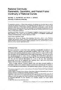
i.e., 𝑑𝑖 (δ,1) ≥ 𝑑𝑖 (δ,0). This completes the proof. 4 Application 4.1. GP problem (Grain-box problem) “It has been decided to shift grain from a warehouse to a factory in an open rectangular box of length 𝑥1 meters, width 𝑥2 meters and height 𝑥3 meters. The bottom, side and ends of the box cost $a, $b and $c/𝑚2 respectively. It cost $1 for each round trip of the box. Assuming that the box will have no salvage value, find the minimum cost of transporting d 𝑚3 of grains”



132

𝑥3 m 𝑥2 m 𝑥1 m Figure 1: Grain-box problem.

This problem can be formulated as Min

𝑔0 (x,s) =

𝑑 𝑥1 𝑥2 𝑥3

+a𝑥1 𝑥2 + 2b𝑥1 𝑥3 + 2𝑐𝑥2 𝑥3

(4.12)

Sub to 𝑥1 ≥ 0, 𝑥2 ≥ 0 , 𝑥3 ≥ 0. Let the input values are 2

Table 1 c($/𝑚2 ) 20

2

a($/𝑚 ) 80

b($/𝑚 ) 10

d(𝑚3 ) 80

Case-1 (crisp method): Here the primal problem is 𝑔0 (x) =

Min

80 𝑥1 𝑥2 𝑥3

+80 𝑥1 𝑥2 + 2. 10𝑥1 𝑥3 + 2.20𝑥2 𝑥3

Sub to 𝑥1 ≥ 0, 𝑥2 ≥ 0 , 𝑥3 ≥ 0. Corresponding dual form is 80 𝛿1

80 𝛿2

2.10 𝛿 2.20 𝛿 ) 3( ) 4 𝛿3 𝛿4

Max

d(δ) = ( ) 𝛿1 ( )𝛿2 (

subject to

𝛿1 + 𝛿2 + 𝛿3 +𝛿4 = 1 − 𝛿1 + 𝛿2 + 𝛿3 = 0 − 𝛿1 + 𝛿2 + 𝛿4 = 0 − 𝛿1 + 𝛿3 + 𝛿4 = 0 𝛿1 , 𝛿2 , 𝛿3 , 𝛿4 ≥ 0. 2 5

1 5

1 5

(4.13)

1 5

From (4.13) we get 𝛿1 = , 𝛿2 = , 𝛿3 = , 𝑎𝑛𝑑 𝛿4 = . The optimal solution of the model through the parametric approach is given by 5.80 2 5.80 1 2.5.10 1 2.5.20 1 ) 5 ( 1 )5 ( 1 )5 ( 1 )5 2

𝑑 ∗ (𝛿) = (

From primal dual relation we get 80 𝑥1 𝑥2 𝑥3

= 𝛿1 ⋆ × 𝑑∗ (𝛿),

80 𝑥1 𝑥2 = 𝛿2 ⋆ × 𝑑∗ (𝛿), 2. 10𝑥1 𝑥3 = 𝛿3 ⋆ × 𝑑∗ (𝛿), 2.20𝑥2 𝑥3 = 𝛿4 ⋆ × 𝑑∗ (𝛿). The optimal solution of the fuzzy model by interval-valued parametric geometric programming is presented in Table 2. Table 2: Optimal Solution of the problem (crisp method) 𝑥1 * 𝑥2 * 𝑥3 * 𝑑 ∗ (𝛿, 𝑠) 𝑔0 (x)* 1 0.5 2 200 200



133

Case- 2 (fuzzy method): When the input data is taken as triangular fuzzy number i.e. 𝑎̃ = (70,80,90), 𝑏̃ = (8,10,12), 𝑐̃ = (16,20,24) and 𝑑̃ = (70,80,90). Using nearest interval approximation method, we get the corresponding interval number and interval-valued function i.e., a = [75,85], ⇒ 𝑎̂ = (75)1−𝑠 (85)𝑠 ∈ [75,85], b = [9,11], ⇒ 𝑏̂ = (9)1−𝑠 (11)𝑠 ∈ [9,11], c = [18,22], ⇒ 𝑐̂ = (18)1−𝑠 (22)𝑠 ∈ [18,22], d = [75,85], ⇒ 𝑑̂ = (75)1−𝑠 (85)𝑠 ∈ [75,85], where s ∈ [0,1]. Here the primal problem is Min

𝑔0 (x,s) =

(75)1−𝑠 (85)𝑠 𝑥1 𝑥2 𝑥3

+(75)1−𝑠 (85)𝑠 𝑥1 𝑥2 + 2(9)1−𝑠 (11)𝑠 𝑥1 𝑥3 + 2(18)1−𝑠 (22)𝑠 𝑥2 𝑥3

Sub to 𝑥1 ≥ 0, 𝑥2 ≥ 0 , 𝑥3 ≥ 0. Corresponding dual form is (75)1−𝑠 (85)𝑠 𝛿 (75)1−𝑠 (85)𝑠 𝛿 2(9)1−𝑠 (11)𝑠 𝛿 2(18)1−𝑠 (22)𝑠 𝛿 ) 1( ) 2( ) 3( ) 4, 𝛿1 𝛿2 𝛿3 𝛿4

Max

d(δ,s) = (

subject to

𝛿1 + 𝛿2 + 𝛿3 +𝛿4 = 1, − 𝛿1 + 𝛿2 + 𝛿3 = 0, − 𝛿1 + 𝛿2 + 𝛿4 = 0, − 𝛿1 + 𝛿3 + 𝛿4 = 0, 𝛿1 , 𝛿2 , 𝛿3 , 𝛿4 ≥ 0. 2 5

1 5

1 5

(4.14)

1 5

From (4.14) we get 𝛿1 = , 𝛿2 = , 𝛿3 = , 𝑎𝑛𝑑 𝛿4 = . The optimal solution of the model through the parametric approach is given by 5(75)1−𝑠 (85)𝑠 2 5(75)1−𝑠 (85)𝑠 1 2×5(9)1−𝑠 (11)𝑠 1 2×5(18)1−𝑠 (22)𝑠 1 ) 5( )5 ( )5 ( )5 2 1 1 1

𝑑 ∗ (𝛿, 𝑠) = (

From primal dual relation we get (75)1−𝑠 (85)𝑠 𝑥1 𝑥2 𝑥3 1−𝑠

= 𝛿1 ⋆ × 𝑑∗ (𝛿, 𝑠),

(75) (85)𝑠 𝑥1 𝑥2 = 𝛿2 ⋆ × 𝑑∗ (𝛿, 𝑠), 2(9)1−𝑠 (11)𝑠 𝑥1 𝑥3 = 𝛿3 ⋆ × 𝑑∗ (𝛿, 𝑠), 2(18)1−𝑠 (22)𝑠 𝑥2 𝑥3 = 𝛿4 ⋆ × 𝑑 ∗ (𝛿, 𝑠). The optimal solution of the fuzzy model by interval-valued parametric geometric programming is presented in Table 3.

s 0.0 0.2 0.4 0.6 0.8 1.0

Table 3: Optimal Solution of the model (fuzzy method) 𝑥1 * 𝑥2 * 𝑥3 * 𝑑 ∗ (𝛿, 𝑠) 0.991 0.496 2.066 184.463 0.995 0.497 2.042 190.285 0.997 0.499 2.017 196.291 1.000 1.004 1.007

0.500 0.502 0.503

1.992 1.964 1.945

202.486 208.876 215.469

𝑔0 (x,s)* 184.463 190.285 196.291 202.486 208.876 215.469

If we compare crisp solution and fuzzy solution, we see that 𝑔0 (x,s)* ≤ 𝑔0 (x)*for s≤ 4, and 𝑔0 (x,s)* ≥ 𝑔0 (x)* for s≥ 6. 4.2. MGP problem (Multi-Grain-box problem) Suppose that to shift grains from a warehouse to a factory in a finite number (say n) of open rectangular boxes of lengths 𝑥1𝑖 meters, widths 𝑥2𝑖 meters and heights 𝑥3𝑖 meters (i=1,2,….,n). The bottom, side and



134

ends of the box cost $𝑎𝑖 , $𝑏𝑖 and $𝑐𝑖 /𝑚2 respectively. It cost $1 for each round trip of the box. Assuming that the box will have no salvage value, find the minimum cost of transporting 𝑑𝑖 𝑚3 of grains.

𝒙𝟏𝟑 𝒙𝟏𝟐

𝒙𝟐𝟑 𝒙𝟏𝟏

𝒙𝟐𝟐 𝒙𝟐𝟏 Figure 2: Multi-Grain-box problem.

This problem can be formulated as an unconstrained MGP problem Min

𝑔0 (x,s) = ∑𝑛𝑖=1(𝑥

𝑑𝑖 1𝑖 𝑥2𝑖 𝑥3𝑖

+ ai 𝑥1𝑖 𝑥2𝑖 + 2bi 𝑥1𝑖 𝑥3𝑖 + 2𝑐𝑖 𝑥2𝑖 𝑥3𝑖 )

(4.15)

Sub to 𝑥1𝑖 ≥ 0, 𝑥2𝑖 ≥ 0 , 𝑥3𝑖 ≥ 0. (i=1,2…..,n). In particular here we assume that the transporting 𝑑𝑖 𝑚3 of grains by the two different open rectangular boxes whose bottom, sides, and the ends of each box costs are give in table 4. Table 4 𝑏𝑖 ($/𝑚2 ) 10 20

𝑎𝑖 ($/𝑚2 ) 80 60

i th Box i=1 i=2

𝑐𝑖 ($/𝑚2 ) 20 30

d(𝑚3 ) 80 50

Case-1 (crisp method): Here the primal problem is ∑2𝑖=1

𝑑𝑖 𝑥𝑖1 𝑥𝑖2 𝑥𝑖3

Min

𝑔0 (x) =

+ 𝑎𝑖 𝑥𝑖1 𝑥𝑖2 + 2𝑏𝑖 𝑥1 𝑥3 + 2𝑐𝑖 𝑥𝑖2 𝑥𝑖3

Sub to

𝑥𝑖1 ≥ 0, 𝑥𝑖2 ≥ 0 , 𝑥𝑖3 ≥ 0.

(4.16)

Corresponding dual form is 𝑑

𝑎

2𝑏

2𝑐

Max

d(𝛿) = ∏2𝑖=1(𝛿 𝑖 )𝛿𝑖1 (𝛿 𝑖 )𝛿𝑖2 ( 𝛿 𝑖)𝛿𝑖3 (𝛿 𝑖)𝛿𝑖4

subject to

𝛿11 + 𝛿12 + 𝛿13 +𝛿14 = 1, 𝛿11 + 𝛿12 + 𝛿13 +𝛿14 = 1, − 𝛿11 + 𝛿12 + 𝛿13 = 0, − 𝛿11 + 𝛿12 + 𝛿13 = 0, − 𝛿11 + 𝛿12 + 𝛿14 = 0, − 𝛿11 + 𝛿12 + 𝛿14 = 0, − 𝛿11 + 𝛿13 + 𝛿14 = 0, − 𝛿11 + 𝛿13 + 𝛿14 = 0, 𝛿11 , 𝛿12 , 𝛿13 , 𝛿14 𝛿21 , 𝛿22 , 𝛿23 , 𝛿24 ≥ 0.

𝑖1

𝑖2

2

𝑖3

1

(4.17)

𝑖4

1

1

2

1

1

1

From (4.17) we get 𝛿11 = 5 , 𝛿12 = 5 , 𝛿13 = 5 , 𝛿14 = 5, 𝛿21 = 5 , 𝛿22 = 5 , 𝛿23 = 5 𝑎𝑛𝑑 𝛿24 = 5 . The optimal solution of the model through the parametric approach is given by 2

∗

𝑑 (𝛿) =

1

1

5.80 5 5.80 5 2.5.10 5 ( 2 ) ( 1 ) ( 1 )

1

2.5.20 5.50 2 5.50 1 2.5.20 1 2.5.30 1 5 ( 1 ) ( 2 ) 5 ( 1 )5 ( 1 )5 ( 1 )5

From primal dual relation we get


Journal of Fuzzy Set Valued Analysis 2016 No. 2 (2016) 125-139 http://www.ispacs.com/journals/jfsva/2016/jfsva-00301/ 80 𝑥11 𝑥12 𝑥13

135

= 𝛿11 ⋆ × 2√𝑑∗ (𝛿),

80 𝑥11 𝑥12 = 𝛿12 ⋆ × 2√𝑑∗ (𝛿), 2. 10𝑥11 𝑥13 = 𝛿13 ⋆ × 2√𝑑∗ (𝛿), 2.20𝑥12 𝑥13 = 𝛿14 ⋆ × 2√𝑑∗ (𝛿), 50 𝑥21 𝑥22 𝑥23

= 𝛿21 ⋆ × 2√𝑑∗ (𝛿),

60 𝑥21 𝑥22 = 𝛿22 ⋆ × 2√𝑑∗ (𝛿), 2. 20𝑥21 𝑥23 = 𝛿23 ⋆ × 2√𝑑∗ (𝛿), 2.30𝑥22 𝑥23 = 𝛿24 ⋆ × 2√𝑑∗ (𝛿). The optimal solution of the fuzzy model by interval-valued parametric geometric programming is presented in Table 5. 𝑥11 * 1.026

𝑥12 * 0.513

Table 5: Optimal Solution of the Model (crisp method): 𝑥13 * 𝑥21 * 𝑥22 * 𝑥23 * 2.053 0.962 0.639 0.961

𝑑 ∗ (𝛿) 38980

𝑔0 (x)* 393.618

Case- 2 (fuzzy method): When the input data are taken as triangular fuzzy numbers i.e., 𝑎̃1 = (70,80,90), 𝑎̃2 = (50,60,70), 𝑏̃1 = (8,10,12), 𝑏̃2 = (16,20,24), 𝑐̃1= (16,20,24), 𝑐̃2= (26,30,34) and 𝑑̃1 = (70,80,90), 𝑑̃2 = (40,50,60). Using nearest interval approximation method, we get the corresponding interval number and interval-valued function i.e., 𝑎̃1 = [75,85], ⇒ 𝑎̂1 = (75)1−𝑠 (85)𝑠 ∈ [75,85], 𝑎̃2 = [75,85], ⇒ 𝑎̂2 = (55)1−𝑠 (65)𝑠 ∈ [55,65], 𝑏̃1 = [9,11], ⇒ 𝑏̂1 = (9)1−𝑠 (11)𝑠 ∈ [9,11], 𝑏̃2 = [18,22], ⇒ 𝑏̂2 = (18)1−𝑠 (22)𝑠 ∈ [18,22], 𝑐̃1 = [18,22], ⇒ 𝑐̂1 = (18)1−𝑠 (22)𝑠 ∈ [18,22], 𝑐̃2 = [28,32], ⇒ 𝑐̂2 = (28)1−𝑠 (32)𝑠 ∈ [28,32], 𝑑̃1 = [75,85], ⇒ 𝑑̂1 = (75)1−𝑠 (85)𝑠 ∈ [75,85], 𝑑̃2 = [45,55], ⇒ 𝑑̂2 = (45)1−𝑠 (55)𝑠 ∈ [45,55], where s ∈ [0,1]. Here the primal problem is 𝑑̂𝑖 𝑥𝑖1 𝑥𝑖2 𝑥𝑖3

+ 𝑎̂𝑖 𝑥𝑖1 𝑥𝑖2 + 2𝑏̂𝑖 𝑥1 𝑥3 + 2𝑐̂𝑖 𝑥𝑖2 𝑥𝑖3

Min

𝑔0 (x,s) = ∑2𝑖=1

Sub to

𝑥𝑖1 ≥ 0, 𝑥𝑖2 ≥ 0 , 𝑥𝑖3 ≥ 0.

(4.18)

Corresponding dual form is 𝑑̂

𝑎̂

2𝑏̂

2𝑐̂

Max

𝑑𝑖 (𝛿, 𝑠) = ∏2𝑖=1(𝛿 𝑖 )𝛿𝑖1 (𝛿 𝑖 )𝛿𝑖2 ( 𝛿 𝑖)𝛿𝑖3 (𝛿 𝑖)𝛿𝑖4

subject to

𝛿11 + 𝛿12 + 𝛿13 +𝛿14 = 1 𝛿11 + 𝛿12 + 𝛿13 +𝛿14 = 1 − 𝛿11 + 𝛿12 + 𝛿13 = 0 − 𝛿11 + 𝛿12 + 𝛿13 = 0 − 𝛿11 + 𝛿12 + 𝛿14 = 0 − 𝛿11 + 𝛿12 + 𝛿14 = 0 − 𝛿11 + 𝛿13 + 𝛿14 = 0 − 𝛿11 + 𝛿13 + 𝛿14 = 0 𝛿11 , 𝛿12 , 𝛿13 , 𝛿14 𝛿21 , 𝛿22 , 𝛿23 , 𝛿24 ≥ 0.

𝑖1

2

𝑖2

1

𝑖3

1

(4.19)

𝑖4

1

2

1

1

1

From (4.19) we get 𝛿11 = 5 , 𝛿12 = 5 , 𝛿13 = 5 , 𝛿14 = 5, 𝛿21 = 5 , 𝛿22 = 5 , 𝛿23 = 5 𝑎𝑛𝑑 𝛿24 = 5 . The optimal solution of the model through the parametric approach is given by


Journal of Fuzzy Set Valued Analysis 2016 No. 2 (2016) 125-139 http://www.ispacs.com/journals/jfsva/2016/jfsva-00301/ 2

∗

𝑑𝑖 (𝛿, 𝑠)

136

1

1

1

5(75)1−𝑠 (85)𝑠 5 5(75)1−𝑠 (85)𝑠 5 2×5(9)1−𝑠 (11)𝑠 5 2×5(18)1−𝑠 (22)𝑠 5 =( ) ( ) ( ) ( ) 2 1 1 1 2 1 1 1 1−𝑠 𝑠 1−𝑠 𝑠 1−𝑠 𝑠 1−𝑠 𝑠 5(45) (55) 5(55) (65) 2×5(18) (22) 2×5(28) (32) ×( ) 5( )5 ( )5 ( )5 2 1 1 1

From primal dual relation we get (75)1−𝑠 (85)𝑠 𝑥11 𝑥12 𝑥13

= 𝛿11 ⋆ × √𝑑𝑖 ∗ (𝛿, 𝑠), 2

(75)1−𝑠 (85)𝑠 𝑥11 𝑥12 = 𝛿12 ⋆ × √𝑑𝑖 ∗ (𝛿, 𝑠), 2

2(9)1−𝑠 (11)𝑠 𝑥11 𝑥13 = 𝛿13 ⋆ × √𝑑𝑖 ∗ (𝛿, 𝑠), 2

2(18)1−𝑠 (22)𝑠 𝑥12 𝑥13 = 𝛿14 ⋆ × √𝑑𝑖 ∗ (𝛿, 𝑠), 2

(45)1−𝑠 (55)𝑠 𝑥21 𝑥22 𝑥23

= 𝛿21 ⋆ × √𝑑𝑖 ∗ (𝛿, 𝑠), 2

(55)1−𝑠 (65)𝑠 𝑥21 𝑥22 = 𝛿22 ⋆ × √𝑑𝑖 ∗ (𝛿, 𝑠), 2

2(18)1−𝑠 (22)𝑠 𝑥21 𝑥23 = 𝛿23 ⋆ × √𝑑𝑖 ∗ (𝛿, 𝑠), 2

2(28)1−𝑠 (32)𝑠 𝑥22 𝑥23 = 𝛿24 ⋆ × √𝑑𝑖 ∗ (𝛿, 𝑠). The optimal solution of the fuzzy model by interval-valued parametric geometric programming is presented in Table 6. 2

Table 6: Optimal Solution of the Model (fuzzy model):

s

𝑥11

*

𝑥12 *

𝑥13 *

𝑥21 *

𝑥22 *

𝑥23 *

𝑔0 (x,s)*

0

1.032

0.516

2.149

0.963

0.619

0.946

363.489

0.2

1.030

0.515

2.112

0.963

0.627

0.952

375.474

0.4

1.027

0.514

2.077

0.962

0.635

0.958

387.917

0.6

1.025

0.513

2.042

0.962

0.644

0.964

400.820

0.8

1.023

0.512

2.007

0.962

0.652

0.970

414.233

1.0

1.021

0.511

1.975

0.961

0.661

0.976

428.160

If we compare crisp solution and fuzzy solution, we see that 𝑔𝑖 (x,s)* ≤ 𝑔𝑖 (x)*for s≤ 4, and 𝑔𝑖 (x,s)* ≥ 𝑔𝑖 (x)* for, s≥ 6. Verify the Theorem. 3.5 in MGP problem (Multi-Grain-box problem): Table 7

s

𝑔0 (x,s)*

𝑑𝑖 ∗ (𝛿, 𝑠)

2 2√di (δ, s)

0 0.2 0.4 0.6 0.8 1.0

363.489 375.474 387.917 400.820 414.233 428.160

32713.23 34986.31 37417.33 40017.26 42797.86 45771.67

361.736 374.093 386.871 400.086 413.753 427.886



137

From the table we see that 𝑔0 (x,s)*≥ 2 2√di (δ, s) for all s ∈ [0,1], so the Theorem 3.5 is verified. For s=0, the lower bound of the interval value of the parameter is used to find the optimal solution. For s=1, the upper bound of interval value of the parameter is used for the optimal solution. These results yield the lower and upper bounds of the optimal solution. The main advantage of the proposed technique is that one can get the intermediate optimal result using proper value s. 5 Conclusion The advantage of this technique is that we can find directly optimal solution of the objective function without solving two-level mathematical programs. This method is simple and takes minimal time. In this paper, we developed unconstrained fuzzy parametric geometric programming problem. In fuzzy we have considered triangular fuzzy number (T.F.N). In future, the other type of membership functions such as piecewise linear hyperbolic, L-R fuzzy number, Trapezoidal Fuzzy Number (TrFN), Parabolic flat Fuzzy Number (PfFN), Parabolic Fuzzy Number (pFN), pentagonal fuzzy number, etc., can be considered to construct the membership function and then model can be easily solved. Acknowledgements The authors are thankful to University of Kalyani for providing financial assistance through DST-PURSE Programme. The authors are grateful to the reviewers for their comments and suggestions. References [1] R. E. Bellman, L. A. Zadeh, Decision making in a fuzzy environment, Management Science, 17 (1970) B141-B164. http://dx.doi.org/10.1287/mnsc.17.4.B141 [2] B. Y. Cao, The further study of posynomial GP with Fuzzy co-e_cient, Mathematics Applicata, 5 (4) (1992) 119-120. [3] C. Carlsson, P. Korhonen, A parametric approach to fuzzy linear programming, Fuzzy sets and systems, (1986) 17-30. http://dx.doi.org/10.1016/S0165-0114(86)80028-8 [4] A. J. Clark, An informal survey of multy-echelon inventory theory, Naval research logistics Quarterly, 19 (1972) 621-650. http://dx.doi.org/10.1002/nav.3800190405 [5] D. Dutta, Pavan Kumar, Fuzzy inventory without shortages using trapezoidal fuzzy number with sensitivity analysis, IOSR Journal of mathematics, 4 (3) (2012) 32-37. http://dx.doi.org/10.9790/5728-0433237 [6] D. Dutta, J. R. Rao, R. N Tiwary, Effect of tolerance in fuzzy linear fractional Programming, Fuzzy sets and systems, 55 (1993) 133-142. http://dx.doi.org/10.1016/0165-0114(93)90126-3 [7] R. J. Duffi, E. L. Peterson, C. M. Zener, Geometric programming- theory and applications, Wiley, New York, (1967).



138

[8] H. Hamacher, H. Leberling, H. J. Zimmermann, Sensitivity Analysis in fuzzy linear Programming, Fuzzy sets and systems, 1 (1978) 269-281. http://dx.doi.org/10.1016/0165-0114(78)90018-0 [9] G. Hadley, T. M. White, Analysis of inventory system, Prentice-Hall, Englewood Cliffs, Nj (1963). [10] Kotb A. M Kotb, Hala A. Fergancy, Multi-item EOQ model with both demand-depended unit cost and varying Leadtime via Geometric Programming, Applied mathematics, 2 (2011) 551-555. http://dx.doi.org/10.4236/am.2011.25072 [11] H. W Khun, A. W. Tucker, Non-linear programming, proceeding second Berkeley symposium Mathematical Statistic and probability (ed) Nyman, J. University of California press, (1951) 481-492. [12] H. X. Li, V. C. Yen, Fuzzy Sets and Fuzzy decision making, CRC press, London (1995). [13] S. T. Liu, Posynomial geometric programming with interval exponents and Coefficients, European Journal of Operational Research, 186 (1) (2008) 17-27. http://dx.doi.org/10.1016/j.ejor.2007.01.031 [14] M. K. Maity, Fuzzy inventory model with two ware house under possibility measure in fuzzy goal, Euro. J. Oper. Res, 188 (1931) 746-774. http://dx.doi.org/10.1016/j.ejor.2007.04.046 [15] F. E. Raymond, Quantity and Economic in manufacturing, McGraw-Hill, New York (1931). [16] S. Dey, T. K. Roy, Optimum shape design of structural model with imprecise coefficient by parametric geometric programming, Decision Science Letters, 4 (2015) 407-418. http://dx.doi.org/10.5267/j.dsl.2015.3.002 [17] S. Islam, T. K. Roy, Modified Geometric programming problem and its applications, J. Appt. Math and computing, 17 (1-2) (2005) 121-144. http://dx.doi.org/10.1007/BF02936045 [18] S. Islam, T. K. Roy, A fuzzy EPQ model with flexibility and reliability consideration and demand depended unit Production cost under a space constraint: A fuzzy geometric programming approach, Applied Mathematics and Computation, 176 (2) (2006) 531-544. http://dx.doi.org/10.1016/j.amc.2005.10.001 [19] S. Islam, T. K. Roy, Multi-Objective Geometric-Programming Problem and its Application, Yugoslav Journal of Operations Research, 20 (2010) 213-227. http://dx.doi.org/10.2298/YJOR1002213I [20] S. T. Liu, Posynomial Geometric-Programming with interval exponents and co-efficients, Europian Journal of Operations Research, 168 (2) (2006) 345-353. http://dx.doi.org/10.1016/j.ejor.2004.04.046 [21] T. K. Roy, M. Maity, A fuzzy inventory model with constraints, Opsearch, 32 (4) (1995) 287-298.



139

[22] W. A. Mandal, S. Islam, Fuzzy Inventory Model for Deteriorating Items, with Time Depended Demand, Shortages, and Fully Backlogging, Pak.j.stat.oper.res. XII (1) (2016) 101-109. [23] W. A. Mandal, S. Islam, Fuzzy Inventory Model for Power Demand Pattern with Shortages, Inflation Under Permissible Delay in Payment, International Journal of Inventive Engineering and Sciences (IJIES), 3 (8) (2015). http://www.ijies.org/attachments/File/v3i8/H0646073815.pdf [24] W. A. Mandal, S. Islam, Fuzzy Inventory Model for Weibull Deteriorating Items, with Time Depended Demand, Shortages, and Partially Backlogging, International Journal of Engineering and Advanced Technology (IJEAT), 4 (5) (2015). https://www.researchgate.net/publication/304167222 [25] W. A. Mandal, S. Islam, A Fuzzy Two-Warehouse Inventory Model for Power Demand Pattern, Shortages with Partially Backlogged, International Journal of Advanced Engineering and Nano Technology (IJAENT), 2 (8) (2015). [26] W. A. Mandal, S. Islam, A Fuzzy Two-Warehouse Inventory Model for Weibull Deteriorating Items with Constant Demand, Shortages and Fully Backlogging, International Journal of Science and Research (IJSR), (2013). https://www.researchgate.net/publication/304168221 [27] W. A. Mandal, S. Islam, Fuzzy Inventory Model for Power Demand Pattern with Inflation, Shortages under Partially Backlogging, International Journal of Science and Research (IJSR), (2013). https://www.researchgate.net/publication/304167141 [28] Y. Liang, F. Zhou, A two warehouse inventory model for deteriorating items under conditionally permissible delay in Payment, Appl. Math. Model, 35 (2011) 2221-2231. http://dx.doi.org/10.1016/j.apm.2010.11.014 [29] L. A. Zadeh, Fuzzy sets, Information and Control, 8 (1965) 338-353. http://dx.doi.org/10.1016/S0019-9958(65)90241-X [30] H. J. Zimmermann, Application of fuzzy set theory to mathematical programming, Information Science, 36 (1985) 29-58. http://dx.doi.org/10.1016/0020-0255(85)90025-8 [31] H. J. Zimmermann, Methods and applications of Fuzzy Mathematical programming, in An introduction to Fuzzy Logic Application in Intelligent Systems, (R. R. Yager and L.A.Zadeh, eds), Kluwer publishers, Boston, (1992) 97- 120. http://dx.doi.org/10.1007/978-1-4615-3640-6_5


Fuzzy unconstrained Parametric Geometric

Fuzzy unconstrained Parametric Geometric

Suggest Documents

223. Fuzzy Parametric Geometric Programming with Application in ...

Geometric characterization and parametric representation of the

Parametric geometric model and shape optimization ...

Robustness of geometric phase under parametric noise

INTEGRATION OF PARAMETRIC GEOMETRIC ... - ITC Digital Library

Parametric Design pattern Language and Geometric ...

ON GEOMETRIC INTERPOLATION BY PLANAR PARAMETRIC ...

Rational Continuity: Parametric, Geometric, and Frenet ... - CiteSeerX

Fuzzy Arithmetic with Parametric LR Fuzzy Numbers - EUSFLAT

Parametric fuzzy sets for automatic color naming

Fuzzy Geometric Programming in Multivariate Stratified Sample ...

Complex Fuzzy Geometric Aggregation Operators - MDPI

Fuzzy Geometric Programming Approach in Multi-objective ...

Interval-Valued Intuitionistic Fuzzy Einstein Geometric Choquet ...

Fuzzy Geometric Programming Optimization using New Arithmetic

A Geometric Framework to Visualize Fuzzy-clustered

Parametric Geometric Modeling of a Spur Gear Using ...

Parametric estimation for the standard and geometric telegraph ...

Geometric Model for a Parametric Study of the ...

On two-parametric Esscher transform for geometric CGMY LÃ©vy ...

unconstrained multivariable optimization

Recognition of Unconstrained Malayalam

UNCONSTRAINED MULTIVARIABLE OPTIMIZATION

Predicting students' grades using fuzzy non-parametric regression ...