k-means clustering algorithm [9, 18] based on the wavelet decomposition. Anytime .... Haar wavelet decomposition on time series . Resolution.
P1: OTE/SPH P2: OTE SVNY295-Petrushin November 1, 2006
16:10
4. Multiresolution Clustering of Time Series and Application to Images Jessica Lin, Michail Vlachos, Eamonn Keogh, and Dimitrios Gunopulos
Summary. Clustering is vital in the process of condensing and outlining information, since it can provide a synopsis of the stored data. However, the high dimensionality of multimedia data today presents an insurmountable challenge for clustering algorithms. Based on the well-known fact that time series and image histograms can both be represented accurately in a lower resolution using orthonormal decompositions, we present an anytime version of the k-means algorithm. The algorithm works by leveraging off the multiresolution property of wavelets. The dilemma of choosing the initial centers for k-means is mitigated by assigning the final centers at each approximation level as the initial centers for the subsequent, finer approximation. In addition to casting k-means as an anytime algorithm, our approach has two other very desirable properties. We observe that even by working at coarser approximations, the achieved quality is better than the batch algorithm, and that even if the algorithm is run to completion, the running time is significantly reduced. We show how this algorithm can be suitably extended to chromatic and textural features extracted from images. Finally, we demonstrate the applicability of this approach on the online image search engine scenario.
4.1 Introduction The vast growth of disk technology in the past decade has enabled us to store large multimedia databases, such as audio, video, images, time series, etc. While storage is no longer an impediment, it has become increasingly clear that an interactive process is needed for humans to efficiently browse through the enormous amount of data. Clustering has proven to be an invaluable tool for distinguishing homogeneous object groups and for producing representatives of the discovered clusters. For example, image clustering is essential for many applications, such as geospatial applications (aerial and satellite photographs), medicine (distinction of tumor images), robot vision (object recognition), online searching (annotation of images), etc. In addition to the high dimensionality of such data, one has to be careful in extracting features that are coherent with the human perceptual system. Such features include, but are not limited to, color, texture, shape, and location. Essentially, the objective is to select content descriptors that are tailored to a specific application and will lead to discovery of homochromous or homomorphic objects.
58
P1: OTE/SPH P2: OTE SVNY295-Petrushin November 1, 2006
16:10
4. Multiresolution Clustering of Time Series and Application to Images
59
Although numerous clustering algorithms have been proposed, the majority of them work in a batch fashion, thus hindering interaction with the end users. Here we address the clustering problem by introducing a novel anytime version of the popular k-means clustering algorithm [9, 18] based on the wavelet decomposition. Anytime algorithms are valuable for large databases, since results are produced progressively and are refined over time [11]. Their utility for data mining has been documented at length elsewhere [2, 20]. While k-means algorithm and wavelet decompositions have both been studied extensively in the past, the major novelty of our approach is that it mitigates the problem associated with the choice of initial centers, in addition to providing the functionality of user interaction. The algorithm works by leveraging off the multiresolution property of wavelets [6]. In particular, an initial clustering is performed with a very coarse representation of the data. The results obtained from this “quick and dirty” clustering are used to initialize a clustering at a finer level of approximation. This process is repeated until the “approximation” is the original “raw” data or until the clustering results stabilize. Furthermore, our approach allows the user to interrupt and terminate the process at any level. In addition to casting the k-means algorithm as an anytime algorithm, our approach has two other very unintuitive properties. The quality of the clustering is often better than the batch algorithm, and even if the algorithm is run to completion, the time taken is typically much less than the time taken by the batch algorithm. We first formulate it as a generic time series problem, since the histograms we extract from images can be well treated as time series. In particular, the high dimensionality and high feature correlation suggest that a time-series algorithm can be suitably applied to image histograms. In this setting, we illustrate the speedup and scalability of the algorithm, in addition to its improved accuracy. Then we show how this novel algorithm can be applied on histograms extracted from image colors and texture. In addition, we demonstrate how a clustering postfiltering step can enhance the interpretability of the results from online image search engines. The rest of this paper is organized as follows. In Section 4.2, we review related work, and introduce the necessary background on the wavelet transform and k-means clustering. In Section 4.3, we introduce our algorithm. Section 4.4 contains a comprehensive comparison of our algorithm to classic k-means on real data sets. In Section 4.5, we apply the algorithm on image data. Section 4.6 summarizes our findings and offers suggestions for future work.
4.2 Background and Related Work Since our work draws on the confluence of clustering, wavelets, and anytime algorithms, we provide the necessary background on these areas in this section. 4.2.1 Background on Clustering One of the most widely used clustering approaches is hierarchical clustering, due to the great visualization power it offers [14]. Hierarchical clustering produces a nested
P1: OTE/SPH P2: OTE SVNY295-Petrushin November 1, 2006
60
16:10
Jessica Lin et al. Table 4.1. An outline of the k-means algorithm Algorithm k-means 1. Decide on a value for k. 2. Initialize the k cluster centers (randomly, if necessary). 3. Decide the class memberships of the N objects by assigning them to the nearest cluster center. 4. Reestimate the k cluster centers, by assuming that the memberships found above are correct. 5. If none of the N objects changed membership in the last iteration, exit. Otherwise go to 3.
hierarchy of similar groups of objects, according to a pairwise distance matrix of the objects. One of the advantages of this method is its generality, since the user does not need to provide any parameters such as the number of clusters. However, its application is limited to only small data sets, due to its quadratic (or higher order) computational complexity. A faster method to perform clustering is k-means [2, 18]. The basic intuition behind k-means (and a more general class of clustering algorithms known as iterative refinement algorithms) is shown in Table 4.1. The k-means algorithm for N objects has time complexity of O(kNrD) [18], with k the number of clusters specified by the user, r the number of iterations until convergence, and D the dimensionality of the points. The shortcomings of the algorithm are its tendency to favor spherical clusters, and the fact that the knowledge on the number of clusters, k, is required in advance. The latter limitation can be mitigated by placing the algorithm in a loop, and attempting all values of k within a large range. Various statistical tests can then be used to determine which value of k is most parsimonious. Since k-means is essentiality a hill-climbing algorithm, it is guaranteed to converge on a local but not necessarily global optimum. In other words, the choices of the initial centers are critical to the quality of results. Nevertheless, in spite of these undesirable properties, for clustering large data sets of time-series, k-means is preferable due to its faster running time. In order to scale the various clustering methods to massive data sets, one can either reduce the number of objects, N , by sampling [2], or reduce the dimensionality of the objects [1, 3, 8, 14, 15, 17, 19, 24, 25]. In the case of time series, the objective is to find a representation at a lower dimensionality that preserves the original information and describes the original shape of the time-series data as closely as possible. Many approaches have been suggested in the literature, including the Discrete Fourier Transform (DFT) [1, 8], Singular Value Decomposition [17], Adaptive Piecewise Constant Approximation [15], Piecewise Aggregate Approximation (PAA) [4, 25], Piecewise Linear Approximation [14], and the Discrete Wavelet Transform (DWT) [3, 19]. While all these approaches have shared the ability to produce a high-quality reduced-dimensionality approximation of time series, wavelets are unique in that their representation of data is intrinsically multiresolution. This property is critical to our proposed algorithm and will be discussed in detail in the next section.
P1: OTE/SPH P2: OTE SVNY295-Petrushin November 1, 2006
16:10
4. Multiresolution Clustering of Time Series and Application to Images
61
Fig. 4.1. The Haar Wavelet can represent data at different levels of resolution. Above we see a raw time series, with increasing faithful wavelet approximations below
Although we choose the Haar wavelet for this work, the algorithm can generally utilize any wavelet basis. The preference for the Haar wavelet is mainly based on its simplicity and its wide usage in the data mining community. 4.2.2 Background on Wavelets Wavelets are mathematical functions that represent data or other functions in terms of the averages and differences of a prototype function, called the analyzing or mother wavelet [6]. In this sense, they are similar to the Fourier transform. One fundamental difference is that wavelets are localized in time. In other words, some of the wavelet coefficients represent small, local subsections of the data being studied, as opposed to Fourier coefficients, which always represent global contributions to the data. This property is very useful for multiresolution analysis of data. The first few coefficients contain an overall, coarse approximation of the data; additional coefficients can be perceived as “zooming-in” to areas of high detail. Figure 4.1 illustrates this idea. The Haar Wavelet decomposition works by averaging two adjacent values on the time series function at a given resolution to form a smoothed, lower dimensional signal, and the resulting coefficients are simply the differences between the values and their averages [3]. The coefficients can also be computed by averaging the differences between each pair of adjacent values. The coefficients are crucial for reconstructing the original sequence, as they store the detailed information lost in the smoothed signal. For example, suppose that we have a time series data T =. Table 4.2 shows the decomposition at different resolutions. As a result, the Haar wavelet decomposition is the collection of the coefficients at all resolutions, with the Table 4.2. Haar wavelet decomposition on time series Resolution 8 4 2 1
Averages 5
Differences (coefficients) < −3 −2 1 −2> −1
P1: OTE/SPH P2: OTE SVNY295-Petrushin November 1, 2006
62
16:10
Jessica Lin et al.
overall average being its first component: . It is clear to see that the decomposition is completely reversible and the original sequence can be reconstructed from the coefficients. For example, to get the signal of the second level, simply compute 5 ± (−1) =< 4, 6 >. Recently there has been an explosion of interest in using wavelets for time series data mining. Researchers have introduced several non-Euclidean, wavelet-based distance measures [13, 22]. Chan and Fu [3] have demonstrated that Euclidean distance indexing with wavelets is competitive to Fourier-based techniques [8]. 4.2.3 Background on Anytime Algorithms Anytime algorithms are algorithms that trade execution time for quality of results [11]. In particular, an anytime algorithm always has a best-so-far answer available, and the quality of the answer improves with execution time. The user may examine this answer at any time, and choose to terminate the algorithm, temporarily suspend the algorithm, or allow the algorithm to run to completion. The usefulness of anytime algorithms for data mining has been extensively documented [2, 20]. Suppose a batch version of an algorithm takes a week to run (not an implausible scenario in data mining massive data sets). It would be highly desirable to implement the algorithm as an anytime algorithm. This would allow a user to examine the best current answer after an hour or so as a “sanity check” of all assumptions and parameters. As a simple example, suppose that the user had accidentally set the value of k to 50 instead of the desired value of 5. Using a batch algorithm, the mistake would not be noted for a week, whereas using an anytime algorithm the mistake could be noted early on and the algorithm restarted with little cost. The motivating example above could have been eliminated by user diligence! More generally, however, data mining algorithms do require the user to make choices of several parameters, and an anytime implementation of k-means would allow the user to interact with the entire data mining process in a more efficient way. 4.2.4 Related Work Bradley et al. [2] suggest a generic technique for scaling the k-means clustering algorithms to large databases by attempting to identify regions of the data that are compressible, that must be retained in main memory, and regions that may be discarded. However, the generality of the method contrasts with our algorithm’s explicit exploitation of the structure of the data type of interest. Our work is more similar in spirit to the dynamic time warping similarity search technique introduced by Chu et al. [4]. The authors speed up linear search by examining the time series at increasingly finer levels of approximation.
4.3 Our Approach—the ik-means Algorithm As noted in Section 4.2.1, the complexity of the k-means algorithm is O(kNrD), where D is the dimensionality of data points (or the length of a sequence, as in the case of
P1: OTE/SPH P2: OTE SVNY295-Petrushin November 1, 2006
16:10
4. Multiresolution Clustering of Time Series and Application to Images
63
time series). For a data set consisting of long time-series, the D factor can burden the clustering task significantly. This overhead can be alleviated by reducing the data dimensionality. Another major drawback of the k-means algorithm derives from the fact that the clustering quality is greatly dependant on the choice of initial centers (i.e., line 2 of Table 4.1). As mentioned earlier, the k-means algorithm guarantees local, but not necessarily global optimization. Poor choices of the initial centers can degrade the quality of clustering solution and result in longer execution time (See [9] for an excellent discussion of this issue). Our algorithm addresses these two problems associated with k-means, in addition to offering the capability of an anytime algorithm, which allows the user to interrupt and terminate the program at any stage. We propose using the wavelet decomposition to perform clustering at increasingly finer levels of the decomposition, while displaying the gradually refined clustering results periodically to the user. We compute the Haar Wavelet decomposition for all time-series data in the database. The complexity of this transformation is linear to the dimensionality of each object; therefore, the running time is reasonable even for large databases. The process of decomposition can be performed offline, and the time-series data can be stored in the Haar decomposition format, which takes the same amount of space as the original sequence. One important property of the decomposition is that it is a lossless transformation, since the original sequence can always be reconstructed from the decomposition. Once we compute the Haar decomposition, we perform the k-means clustering algorithm, starting at the second level (each object at level i has 2(i−1) dimensions) and gradually progress to finer levels. Since the Haar decomposition is completely reversible, we can reconstruct the approximate data from the coefficients at any level and perform clustering on these data. We call the new clustering algorithm ik-means, where i stands for “incremental.” Figure 4.2 illustrates this idea. The intuition behind this algorithm originates from the observation that the general shape of a time series sequence can often be approximately captured at a lower resolution. As shown in Figure 4.1, the shape of the time series is well preserved, even at very coarse approximations. Because of this desirable property of wavelets, clustering results typically stabilize at a low resolution.
Level 1 Points for k-means at level 2
Level 2
Points for k-means at level 3
Level 3
Level n Time series 1
Time series 2
Time series k
Fig. 4.2. k-means is performed on each level on the reconstructed data from the Haar wavelet decomposition, starting with the second level.
P1: OTE/SPH P2: OTE SVNY295-Petrushin November 1, 2006
64
16:10
Jessica Lin et al. Table 4.3. An outline of the ik-means algorithm Algorithm ik-means Decide on a value for k. Initialize the k cluster centers (randomly, if necessary). Run the k-means algorithm on the leveli representation of the data Use final centers from leveli as initial centers for leveli+1 . This is achieved by projecting the k centers returned by k-means algorithm for the 2i space in the 2i+1 space. 5. If none of the N objects changed membership in the last iteration, exit. Otherwise go to 3.
1. 2. 3. 4.
At the end of each level, we obtain clustering results on the approximation data used at the given level. We can therefore use that information to seed the clustering on the subsequent level. In fact, for every level except the starting level (i.e., level 2), which uses random initial centers, the initial centers are selected on the basis of the final centers from the previous level. More specifically, the final centers computed at the end of level i will be used as the initial centers on level i + 1. Since the length of the data reconstructed from the Haar decomposition doubles as we progress to the next level, we project the centers computed at the end of level i onto level i + 1 by doubling each coordinate of the centers. This way, they match the dimensionality of the points on level i + 1. For example, if one of the final centers at the end of level 2 is , then the initial center used for this cluster on level 3 is . This approach mitigates the dilemma associated with the choice of initial centers, which is crucial to the quality of clustering results [9]. It also contributes to the fact that our algorithm often produces better clustering results than the k-means algorithm. The pseudocode of the algorithm is provided in Table 4.3. The algorithm achieves the speedup by doing the vast majority of reassignments (Line 3 in Table 5.1), at the lower resolutions, where the costs of distance calculations are considerably lower. As we gradually progress to finer resolutions, we already start with good initial centers. Therefore, the number of iterations r until convergence will typically be much lower. The ik-means algorithm allows the user to monitor the quality of clustering results as the program executes. The user can interrupt the program at any level, or wait until the execution terminates once it stabilizes. Typically we can consider the process stabilized if the clustering results do not improve for more than two stages. One surprising and highly desirable finding from the experimental results (as shown in the next section) is that even if the program is run to completion (i.e., until the last level, with full resolution), the total execution time is generally less than that of clustering on the raw data. 4.3.1 Experimental Evaluation on Time Series To show that our approach is superior to the k-means algorithm for clustering time series, we performed a series of experiments on publicly available real data sets. For completeness, we ran the ik-means algorithm for all levels of approximation, and recorded the cumulative execution time and clustering accuracy at each level. In
P1: OTE/SPH P2: OTE SVNY295-Petrushin November 1, 2006
16:10
4. Multiresolution Clustering of Time Series and Application to Images
65
reality, however, the algorithm stabilizes in early stages and can be terminated much sooner. We compare the results with that of k-means on the original data. Since both algorithms start with random initial centers, we execute each algorithm 100 times with different centers. However, for consistency we ensure that for each execution, both algorithms are seeded with the same set of initial centers. After each execution, we compute the error (more details will be provided in Section 4.4.2) and the execution time on the clustering results. We compute and report the averages at the end of each experiment. By taking the average, we achieve better objectiveness than taking the best (minimum), since in reality, we would not have the knowledge of the correct clustering results, or the “oracle,” to compare against our results (as in the case with one of our test data sets). 4.3.2 Data Sets and Methodology We tested on two publicly available, real data sets. The data set cardinalities range from 1,000 to 8,000. The length of each time series has been set to 512 on one data set, and 1024 on the other. Each time series is z-normalized to have mean value of 0 and standard deviation of 1. r JPL: This data set consists of readings from various inertial sensors from Space Shuttle mission STS-57. The data are particularly appropriate for our experiments since the use of redundant backup sensors means that some of the data are very highly correlated. In addition, even sensors that measure orthogonal features (i.e., the X- and Y-axis) may become temporarily correlated during a particular maneuver; for example, a “roll reversal” [7]. Thus, the data have an interesting mixture of dense and sparse clusters. To generate data sets of increasingly larger cardinalities, we extracted time series of length 512, at random starting points of each sequence from the original data pool. r Heterogeneous: This data set is generated from a mixture of 10 real-time series data from the UCR Time Series Data Mining Archive [16]. Figure 4.3 shows the 10 time-series we use as seeds. We produced variations of the original patterns by adding small time warping (2–3% of the series length), and interpolated Gaussian noise. Gaussian noisy peaks are interpolated using splines to create smooth random variations. Figure 4.4 shows how data are generated. In the Heterogeneous data set, we know that the number of clusters (k) is 10. However, for the JPL data set, we lack this information. Finding k is an open problem for the k-means algorithm and is out of scope of this chapter. To determine the optimal k for k-means, we attempt different values of k, ranging from 2 to 8. Nonetheless, our algorithm outperforms the k-means algorithm regardless of k. In this chapter we show only the results with k equals to 5. Figure 4.5 shows that our algorithm produces the same results as does the hierarchical clustering algorithm, which is generally more costly. 4.3.3 Error of Clustering Results In this section we compare the clustering quality for the ik-means and the classic k-means algorithm.
P1: OTE/SPH P2: OTE SVNY295-Petrushin November 1, 2006
66
16:10
Jessica Lin et al. Burst
Earthquake
2
2
1
0
Infrasound 0
1
0
200 400 600 800 1000
−4
Memory
−4
−1
−6
−2 200 400 600 800 1000
200 400 600 800 1000
Ocean 2
0 1
−1
0 −1 200 400 600 800 1000
−2
0
−3
−1
Sunspot
Random walk
Power data
0
1
200 400 600 800 1000
1
1
2
−2
0
−2
−1
Koski ecg
2
200 400 600 800 1000
−1 −2 200 400 600 800 1000
200 400 600 800 1000
Tide 3
4
2
2
1 0 −1 −2
0 200 400 600 800 1000
200 400 600 800 1000
Fig. 4.3. Real-time series data from UCR Time Series Data Mining Archive. We use these time series as seeds to create our heterogeneous data set.
Since we generated the heterogeneous data sets from a set of given time series data, we have the knowledge of correct clustering results in advance. In this case, we can simply compute the clustering accuracy by summing up the number of correctly classified objects for each cluster c and then dividing by the data set cardinality. This is done by the use of a confusion matrix. Note the accuracy computed here is equivalent to “recall,” and the error rate is simply ε = 1 – accuracy. The error is computed at the end of each level. However, it is worth mentioning that in reality, the correct clustering information would not be available in advance. The incorporation of such known results in our error calculation merely serves the purpose of demonstrating the quality of both algorithms. For the JPL data set, we do not have prior knowledge of correct clustering information (which conforms more closely to real-life cases). Lacking this information, we cannot use the same evaluation to determine the error. Since the k-means algorithm seeks to optimize the objective function by minimizing the sum of squared intracluster errors, we can evaluate the quality of clustering by using the objective functions. However, since the ik-means algorithm involves data with smaller dimensionality except for the last level, we have to compute the objective functions on the raw data, in order to compare with the k-means algorithm. We show that the objective functions obtained from the ik-means algorithm are better than those from the k-means algorithm. The results are consistent with the work of [5], in which the authors show that dimensionality reduction reduces the chances of
P1: OTE/SPH P2: OTE SVNY295-Petrushin November 1, 2006
16:10
4. Multiresolution Clustering of Time Series and Application to Images Original trajectory 1000
67
Noise − Interpolating Gaussian Peaks 300
800
200
600
100
400
0
200
−100 200
400
600
800 1000
Adding time−shifting 1000
200
400
600
Final Copy = Original + Noise + Time Shift 1200
Final Original
1000
800
800 1000
800 600 600 400
400 200
200 200
400
600
800 1000
200
400
600
800 1000
Fig. 4.4. Generation of variations on the heterogeneous data. We produced variation of the original patterns by adding small time shifting (2–3% of the series length), and interpolated Gaussian noise. Gaussian noisy peaks are interpolated using splines to create smooth random variations. e e e d d d b b b c c c a a a
Fig. 4.5. On the left-hand side, we show three instances from each cluster discovered by the ik-means algorithm. We can visually verify that our algorithm produces intuitive results. On the right-hand side, we show that hierarchical clustering (using average linkage) discovers the exact same clusters. However, hierarchical clustering is more costly than our algorithm.
P1: OTE/SPH P2: OTE SVNY295-Petrushin November 1, 2006
68
16:10
Jessica Lin et al. ik-means error as fraction of k-means (Heterogeneous)
1 Fraction 0.5 0 2
8
32 128
512
8000 4000 Data 2000 1000 size
Dimensionality
Fig. 4.6. Error of ik-means algorithm on the heterogeneous data set, presented as fraction of the error from the k-means algorithm. Our algorithm results in smaller error than the k-means after the second stage (i.e., four dimensions), and stabilizes typically after the third stage (i.e., eight dimensions).
the algorithm being trapped in a local minimum. Furthermore, even with the additional step of computing the objective functions from the original data, the ik-means algorithm still takes less time to execute than the k-means algorithm. In Figures 4.6 and 4.7, we show the errors/objective functions from the ik-means algorithm as a fraction of those obtained from the k-means algorithm. As we can see from the plots, our algorithm stabilizes at early stages and consistently results in smaller error than the classic k-means algorithm. 4.3.4 Running Time In Figures 4.8 and 4.9, we present the cumulative running time for each level on the ik-means algorithm as a fraction to the k-means algorithm. The cumulative running ik-means Obj function as fraction to k-means (JPL)
1.00 Fraction
0.50 0.00 2
8
32
128
512
8000 4000 2000 Data 1000 size
Dimensionality
Fig. 4.7. Objective functions of ik-means algorithm on the JPL data set, presented as fraction of error from the k-means algorithm. Again, our algorithm results in smaller objective functions (i.e., better clustering results) than the k-means, and stabilizes typically after the second stage (i.e., four dimensions).
P1: OTE/SPH P2: OTE SVNY295-Petrushin November 1, 2006
16:10
4. Multiresolution Clustering of Time Series and Application to Images
69
ik-means cumulative time as fraction of k-means (Heterogeneous) 1.2 0.9 Fraction 0.6 0.3 0 2
8
32
128
512
8000 4000 2000 Data 1000 size
Dimensionality
Fig. 4.8. Cumulative running time for the heterogeneous data set. Our algorithm typically cuts the running time by half as it does not need to run through all levels to retrieve the best results.
time for any leveli is the total running time from the starting level (level 2) to level i. In most cases, even if the ik-means algorithm is run to completion, the total running time is still less than that of the k-means algorithm. We attribute this improvement to the good choices of initial centers for successive levels after the starting level, since they result in very few iterations until convergence. Nevertheless, we have already shown in the previous section that the ik-means algorithm finds the best result in relatively early stage and does not need to run through all levels.
4.4 ik-means Algorithm vs. k-means Algorithm In this section (Figs. 4.10 and 4.11), rather than showing the error/objective function on each level, as in Section 4.4.2, we present only the error/objective function returned by the ik-means algorithm when it stabilizes or, in the case of JPL data set, outperforms ik-means cumulative time as fraction to k-means (JPL) 1.00 0.80 0.60 Fraction 0.40 0.20 0.00
2
8
32
128 512
8000 4000 2000 Data 1000 size
Dimensionality
Fig. 4.9. Cumulative running time for the JPL data set. Our algorithm typically takes only 30% of time.
P1: OTE/SPH P2: OTE SVNY295-Petrushin November 1, 2006
70
16:10
Jessica Lin et al. ik-means Alg vs. k-means Alg (heterogeneous) Error 1
Time (s)
0.8
40
0.6
30
0.4
20
0.2
10
50
0
0 1000
2000
4000
8000
Data size error_ik-means
error_k-means
time_ik-means
time_k-means
Fig. 4.10. The ik-means algorithm is highly competitive with the k-means algorithm. The errors and execution time are significantly smaller.
the k-means algorithm in terms of the objective function. We also present the time taken for the ik-means algorithm to stabilize. We compare the results with those of the k-means algorithm. From the figures we can observe that our algorithm achieves better clustering accuracy at significantly faster response time. Figure 4.12 shows the average level where the ik-means algorithm stabilizes or, in the case of JPL, outperforms the k-means algorithm in terms of objective function. Since the length of the time series data is 1024 in the heterogeneous data set, there are 11 levels. Note that the JPL data set has only 10 levels since the length of the time series data is only 512. We skip level 1, in which the data have only one dimension
ik-means Alg vs. k-means Alg (JPL) Obj. Fcn (x10,000)
Time (s) 80
150
60
100
40
50
20
0
1000
2000
4000
8000
0
Data size obj. fcn_ik-means
obj. fcn_k-means
time_ik-means
time_k-means
Fig. 4.11. ik-means vs. k-means algorithms in terms of objective function and running time for JPL data set. Our algorithm outperforms the k-means algorithm. The running time remains small for all data sizes because the algorithm terminates at very early stages.
P1: OTE/SPH P2: OTE SVNY295-Petrushin November 1, 2006
16:10
4. Multiresolution Clustering of Time Series and Application to Images
71
Levels
Avg level until stabilization (1–11) 11 9 7 5 3 1
Heterogeneous JPL
1000
2000 4000 Data size
8000
Fig. 4.12. Average level until stabilization. The algorithm generally stabilizes between level 3 and level 6 for heterogeneous data set, and between level 2 and 4 for the JPL data set.
(the average of the time series) and is the same for all sequences, since the data have been normalized (zero mean). Each level i has 2(i−1) dimensions. From the plot we can see that our algorithm generally stabilizes at levels 3–6 for the heterogeneous data set and at levels 2–4 for the JPL data set. In other words, the ik-means algorithm operates on data with a maximum dimensionality of 32 and 8, respectively, rather than 1024 and 512.
4.5 Application to Images In this section we provide preliminary results regarding the applicability of our approach for images. Image data can be represented as “time” series by combining different descriptors into a long series. Although the notion of “time” does not exist here, a series formed by the descriptors has similar characteristics as time series, namely, high dimensionality and strong autocorrelation. The simplest and perhaps the most intuitive descriptor for images is the color. For each image, a color histogram of length 256 can be extracted from each of the RGB components. These color histograms are then concatenated to form a series of length 786. This series serves as a “signature” of the image and summarizes the image in chromatic space. To demonstrate that this representation of images is indeed appropriate, we performed a simple test run on a small data set. The data set consists of three categories of images from the Corel image database: diving, fireworks, and tigers. Each category contains 20 images. The clustering results are shown in Figure 4.13. As it shows, most images were clustered correctly regardless of the variety presented within each category, except for 2: the last two images in the Fireworks cluster belong to the Tigers cluster. A closer look at the images explains why this happens. These two misclustered Tiger images have relatively dark background compared to the rest of images in the same category, and since we used color histograms, it is understandable that these two images were mistaken as members of the Fireworks cluster. The clustering results show that representing images using merely the color histogram is generally very effective, as it is invariant to rotation and the exact contents
P1: OTE/SPH P2: OTE SVNY295-Petrushin November 1, 2006
72
16:10
Jessica Lin et al.
Fig. 4.13. Clustering results using RGB color descriptor. Two of the Tiger images were misclustered in the fireworks cluster due to similar color decomposition.
P1: OTE/SPH P2: OTE SVNY295-Petrushin November 1, 2006
16:10
4. Multiresolution Clustering of Time Series and Application to Images
73
of the images. However, the misclustering also implies that the color descriptor alone might not be good enough to capture all the essential characteristics of an image and could be limited for images with similar color decomposition. To mitigate this shortcoming, more descriptors such as texture can be used in addition to the color descriptor. In general, the RGB components are highly correlated and do not necessarily coincide with the human visual system. We validate this observation empirically, since our experiments show that a different chromatic model, HSV, generally results in clusters of better quality. For texture, we apply Gabor-wavelet filters [23] at various scales and orientations, which results in an additional vector of size 256. The color and texture information are concatenated and the final vector of size 1024 is treated as a time series. Therefore, the method that we proposed in the previous sections can be applied unaltered to images. Notice that this representation can very easily facilitate a weighted scheme, where according to the desired matching criteria we may favor the color or the texture component. Figure 4.14 shows how the time series is formed from an image. A well-known observation in the image retrieval community is that the use of large histograms suffers from the “curse of dimensionality” [10]. Our method is therefore particularly applicable in this scenario, since the wavelet (or any other) decomposition can help reduce the dimensionality effectively. It should also be noted that the manipulation of
Red or hue
Green or saturation
Blue or value
Texture
100 200 300 400 500 600 700 800 900 1000
Fig. 4.14. An example of the image vector that is extracted for the purposes of our experiments.
P1: OTE/SPH P2: OTE SVNY295-Petrushin November 1, 2006
74
16:10
Jessica Lin et al. Table 4.4. Clustering error and running time averaged over 100 runs. Our method is even more accurate than hierarchical clustering, which requires almost an order of magnitude more time. Error RGB HSV HSV+ TEXTR HSV+ TEXTR+ good centers
Time (s)
Hier. 0.31 0.36 0.24
k-means 0.37 0.26 0.25
ik-means 0.37 0.26 0.19
Hier. 50.7 49.8 55.5
k-means 11.18 11.12 11.33
ik-means 4.94 6.82 3.14
N/A
0.22
0.17
N/A
8.26
2.89
the image features as time series is perfectly valid. The characteristics of “smoothness” and autocorrelation of the time series are evident here, since adjacent bins in the histograms have very similar values. We demonstrate the usefulness of our approach on two scenarios. 4.5.1 Clustering Corel Image Data sets First, we perform clustering on a subset of images taken from the Corel database. The data set consists of six clusters, each containing 100 images. The clusters represent diverse topics: diving, fireworks, tigers, architecture, snow, and stained glass, some of which have been used in the test-run experiment. This is by no means a large data set; however, it can very well serve as an indicator of the speed and the accuracy of the ik-means algorithm. In our case studies, we utilize two descriptors, color and texture, and compare two color representations: RGB and HSV. We compare the algorithm with k-means, and with hierarchical clustering using Ward’s linkage method. Our approach achieves the highest recall rate and is also the fastest method. Since the performance of k-means greatly depends on the initial choice of centers, we also provided “good” initial centers by picking one image randomly from each cluster. Even in this scenario our algorithm was significantly faster and more accurate. The results, shown in Table 4.4, are generated using the L1 distance metric. Although we also tested on the Euclidean distance, using L1 metric generally results in better accuracy for our test cases. The advantages of our algorithm are more evident with large, disk-based data sets. To demonstrate, we generate a larger data set from the one we used in Table 4.4, using the same methodology as described in Figure 4.4. For each image in the data set, we generate 99 copies with slight variations, resulting in a total of 60,000 images (including the original images in the data set). Each image is represented as a time series of length 1024; therefore, it would require almost 500 MB of memory to store the entire data set. Clustering on large data sets is resource-demanding for k-means, and one single run of k-means could take more than 100 iterations to converge. In
P1: OTE/SPH P2: OTE SVNY295-Petrushin November 1, 2006
16:10
4. Multiresolution Clustering of Time Series and Application to Images
75
addition, although it is common for computers today to be equipped with 1 GB or more memory, we cannot count on every user to have the sufficient amount of memory installed. We also need to take into consideration other memory usage required by the intermediate steps of k-means. Therefore, we will simulate the disk-based clustering environment by assuming a memory buffer of a fixed size that is smaller than the size of our data set. Running k-means on disk-based data sets, however, would require multiple disk scans, which is undesirable. With ik-means, such concerns are mitigated. We know from the previous experimental results that ik-means stabilizes on early stages; therefore, in most cases we do not need to operate on the fine resolutions. In other words, we will read in the data at the highest resolution allowed, given the amount of memory available, and if the algorithm stabilizes on these partial-Haar coefficients, then we can stop without having to retrieve the remaining data from the disk. For simplicity, we limit our buffer size to 150 MB, which allows us to read in as much as 256 coefficients (a 4:1 reduction for time series length of 1024). With limited memory resources, we would need to use the disk-based k-means algorithm. However, to make it simple for k-means, we run k-means on the smoothed data with a reduction ratio of 4:1 (i.e., equivalent to the reconstructed time series at the finest resolution of the partial-Haar). Although performing data smoothing prior to k-means aligns more closely to the underlying philosophy of ik-means and is a logical thing to do, it lacks the flexibility of ik-means in terms of data reduction. Overall, ik-means still offers the advantages associated with being multi-resolutional. In fact, our experiment shows that ik-means stabilizes before running on the finest resolution of the partial-Haar coefficients. Since the data set was generated from six clusters, intuitively, we could assume that an image has the same cluster label as the “seed” image that generated it, and that we could evaluate clustering accuracy by comparing the class labels to the correct labels. However, it is also possible that in the data generation process, too much noise is introduced such that the generated image should not belong in the same cluster as the seed image. Though unlikely, as we control the amount of noise to be added such as limiting time shifting to 2–3% of the length of time series data, to avoid any bias, we arbitrarily increase the number of clusters to 10. In this scenario, we compare the projected objective functions instead, as this is the most intuitive way to evaluate k-means clustering. In both scenarios, ik-means achieves higher accuracy than k-means. With k = 6, ik-means outperforms k-means starting at the third level, using only four coefficients which, naturally, also results in shorter running time. With k = 10, however, ik-means outperforms k-means at a later level (level 6), thus resulting in longer running time. 4.5.2 Clustering Google Images For the second paradigm we used a real-world example from the image search feature of Google. All online image search engines gather information based only on key words. Therefore, the image query results can be from very diverse disciplines and have very different content. For example, if one searches for “bass,” the result would be
P1: OTE/SPH P2: OTE SVNY295-Petrushin November 1, 2006
76
16:10
Jessica Lin et al.
Fig. 4.15. Clustering results on the image query “horse” posed at Google
a mixture of images about “fish” and “musical instruments.” Although in some cases we might be able to avoid the ambiguity by supplying more descriptive key words, it is not always trivial to find the right key words that describe exactly the images we have in mind. In this specific case, a postfiltering of the matches using texture features can create separate clusters of images, and as a consequence, lead to a more intuitive presentation of the results. In order for such a postfiltering step to become a reality, it is obvious that one must utilize an extremely lightweight algorithm. We posed several queries on Google and we grouped the results into clusters. Here we present representative results for the word “horse.” The first 20 images are retrieved. The images are passed on to our algorithm and clustered into two groups. Figure 4.15 presents the results. We can see that there is an obvious separation between the handdrawn pictures and the photographic images. These experiments suggest that online image search could be augmented by a clustering step, in the spirit of the well-known “Scatter/Gather” framework [12]. The results could be improved by using relevance feedback. In addition, compact histogram representations, as well as the use of more robust distance functions such
P1: OTE/SPH P2: OTE SVNY295-Petrushin November 1, 2006
16:10
4. Multiresolution Clustering of Time Series and Application to Images
77
as the dLog distance proposed in [21], could further boost the performance for the proposed algorithm.
4.6 Conclusions and Future Work We have presented an approach to perform incremental clustering at various resolutions, using the Haar wavelet transform. Using k-means as our clustering algorithm, we reuse the final centers at the end of each resolution as the initial centers for the next level of approximation. This approach mitigates the dilemma associated with the choices of initial centers for k-means and significantly improves the execution time and clustering quality. Our experimental results indicate that this approach yields faster execution time than the traditional k-means approach, in addition to improving the clustering quality of the algorithm. The anytime algorithm stabilizes at very early stages, eliminating the needs to operate on high dimensionality. In addition, the anytime algorithm allows the user to terminate the program at any stage. Since image histograms extracted from colors and textures can be suitably treated as time series, we further demonstrate the efficacy of our algorithm on the image data. In future work, we plan to examine the possibility of reusing the results (i.e., objective functions that determine the quality of clustering results) from the previous stages to eliminate the need to recompute all the distances.
Acknowledgments We thank B. S. Manjunath and Shawn Newsam for providing the Gabor filter code.
References 1. Agrawal R, Faloutsos C, Swami A. Efficient similarity search in sequence databases. In: Proceedings of the 4th Int’l Conference on Foundations of Data Organization and Algorithms; 1993 Oct 13–15; Chicago, IL; pp. 69–84. 2. Bradley P, Fayyad U, Reina C. Scaling clustering algorithms to large databases. In: Proceedings of the 4th Int’l Conference on Knowledge Discovery and Data Mining; 1998 Aug 27–31; New York, NY, pp. 9–15. 3. Chan K, Fu AW. Efficient time series matching by wavelets. In: Proceedings of the 15th IEEE Int’l Conference on Data Engineering; 1999 Mar 23–26; Sydney, Australia; pp. 126– 133. 4. Chu S, Keogh E, Hart D, Pazzani M. Iterative deepening dynamic time warping for time series. In: Proceedings of the 2nd SIAM International Conference on Data Mining; 2002 Apr 11–13; Arlington, VA. 5. Ding C, He X, Zha H, Simon H. Adaptive dimension reduction for clustering high dimensional data. In: Proceedings of the 2nd IEEE International Conference on Data Mining; 2002 Dec 9–12; Maebashi, Japan, pp. 147–154.
P1: OTE/SPH P2: OTE SVNY295-Petrushin November 1, 2006
78
16:10
Jessica Lin et al.
6. Daubechies I. Ten Lectures on Wavelets. Number 61 in CBMS-NSF regional conference series in applied mathematics, Society for Industrial and Applied Mathematics; 1992; Philadelphia. 7. Dumoulin J. NSTS 1988 News Reference Manual. http://www.fas.org/spp/civil/sts/ 8. Faloutsos C, Ranganathan M, Manolopoulos Y. Fast subsequence matching in time-series databases. In: Proceedings of the ACM SIGMOD Int’l Conference on Management of Data; 1994 May 25–27; Minneapolis, pp. 419–429. 9. Fayyad U, Reina C, Bradley P. Initialization of iterative refinement clustering algorithms. In: Proceedings of the 4th International Conference on Knowledge Discovery and Data Mining; 1998 Aug 27–31; New York, NY; pp. 194–198. 10. Gibson S, Harvey R. Analyzing and simplifying histograms using scale-trees. In: Proceedings of the 11th Int’l Conference on Image Analysis and Processing; 2001 Sept 26–28; Palermo, Italy. 11. Grass J, Zilberstein S. Anytime algorithm development tools. Sigart Artificial Intelligence 1996;7:2. 12. Hearst MA, Pedersen JO. Reexamining the cluster hypothesis: Scatter/gatter on retrieval results. In: Proceedings of the 19th Annual International ACM SIGIR Conference on Research and Development in Information Retrieval; 1996 Aug 18–22; Zurich, Switzerland. 13. Huhtala Y, K¨arkk¨ainen J, Toivonen H. Mining for similarities in aligned time series using wavelets. Data Mining and Knowledge Discovery: Theory, Tools, and Technology. SPIE Proceedings Series 1999; 3695:150–160. Orlando, FL. 14. Keogh E, Pazzani M. An enhanced representation of time series which allows fast and accurate classification, clustering and relevance feedback. In: Proceedings of the 4th Int’l Conference on Knowledge Discovery and Data Mining; 1998 Aug 27–31; New York, NY; pp. 239–241. 15. Keogh E, Chakrabarti K, Pazzani M, Mehrotra S. Locally adaptive dimensionality reduction for indexing large time series databases. In: Proceedings of ACM SIGMOD Conference on Management of Data. 2001 May 21–24; Santa Barbara, CA; pp. 151–162. 16. Keogh E, Folias T. The UCR Time Series Data Mining Archive (http://www.cs.ucr.edu/∼eamonn/TSDMA/index.html). 2002. 17. Korn F, Jagadish H, Faloutsos C. Efficiently supporting ad hoc queries in large datasets of time sequences. In: Proceedings of the ACM SIGMOD Int’l Conference on Management of Data; 1997 May 13–15; Tucson, AZ, pp. 289–300. 18. McQueen J. Some methods for classification and analysis of multivariate observation. In: Le Cam L, Neyman J, eds. 5th Berkeley Symp. Math. Stat. Prob. 1967; 281–297. 19. Popivanov I, Miller RJ. Similarity search over time series data using wavelets. In: Proceedings of the 18th Int’l Conference on Data Engineering; 2002 Feb 26-Mar 1; San Jose, CA, pp. 212–221. 20. Smyth P, Wolpert D. Anytime exploratory data analysis for massive data sets. In: Proceedings of the 3rd Int’l Conference on Knowledge Discovery and Data Mining; 1997 Aug 14–17; Newport Beach, CA, pp. 54–60. 21. Stehling RO, Nascimento MA, Falc˜ao AX. A compact and efficient image retrieval approach based on border/interior pixel classification. In: Proceedings of the ACM Intl. Conf. on Information and Knowledge Management; 2002 Nov 4–9; McLean, VA. 22. Struzik Z, Siebes A. The Haar wavelet transform in the time series similarity paradigm. In: Proceedings of Principles of Data Mining and Knowledge Discovery, 3rd European Conference; 1999 Sept 15–18; Prague, Czech Republic; pp. 12–22.
P1: OTE/SPH P2: OTE SVNY295-Petrushin November 1, 2006
16:10
4. Multiresolution Clustering of Time Series and Application to Images
79
23. Wu P, Manjunath BS, Newsam S, Shin HD. A texture descriptor for browsing and similarity retrieval. Journal of Signal Processing: Image Communication 2000;16:1–2;33–43. 24. Wu Y, Agrawal D, El Abbadi A. A comparison of DFT and DWT based similarity search in time-series databases. In: Proceedings of the 9th ACM CIKM Int’l Conference on Information and Knowledge Management. 2000 Nov 6–11; McLean, VA; pp. 488–495. 25. Yi B, Faloutsos C. Fast time sequence indexing for arbitrary lp norms. In: Proceedings of the 26th Int’l Conference on Very Large Databases; 2000 Sept 10–14; Cairo, Egypt; pp. 385–394.