A comparison of multiple linear regression and quantile regression for modeling the internal bond of medium density fiberboard Timothy M. Young✳ Leslie B. Shaffer Frank M. Guess✳ Halima Bensmail Ramón V. León
Abstract Multiple linear regression (MLR) and quantile regression (QR) models were developed for the internal bond (IB) of medium density fiberboard (MDF). The data set that aligned the IB of MDF came from 184 independent variables that corresponded to online sensors. MLR models were developed for MDF product types that were distinguished by thickness in inches, i.e., 0.750-inch, 0.6875-inch, 0.625-inch, and 0.500-inch. A best model criterion was used with all possible subsets. QR models were developed for each product type for the most common independent variable of the MLR models for comparison. The adjusted coefficient of determination (R2a) of the MLR models ranged from 72 percent with 53 degrees of freedom to 81 percent with 42 degrees of freedom. The Root Mean Square Errors (RMSE) ranged from 6.05 pounds per square inch (psi) to 6.23 psi; the maximum Variance Inflation Factor (VIF) was 5.6, and all residual patterns were homogeneous. A common independent variable for the 0.750-inch and 0.625-inch MLR models was “Refiner Resin Scavenger %.” QR models for 0.750 inch and 0.625 inch indicate similar slopes for the median and average, with different slopes at the fifth and 95th percentiles. “Face Humidity” was a common independent variable for the 0.6875-inch and 0.500-inch MLR models. QR models for 0.6875-inch and 0.500-inch indicate different slopes for the median and average, and instability in IB in the outer fifth and 95th percentiles. The use of QR models to investigate the percentiles of the IB of MDF suggests significant opportunities for manufacturers for continuous improvement and cost savings.
T
he wood composites industry is undergoing unprecedented change in the forms of corporate divestitures and consolidation, real increases in the cost of raw material and energy, and extraordinary international competition. The forest products industry is an important contributor to the U.S. economy. In 2002, this sector contributed more than $240 billion to the economy and employed more than one million Americans in 22,231 primary wood products manufacturing facilities (U.S. Census Bureau 2004). Sustaining business competitiveness by reducing costs and maintaining product quality will be essential for this industry. One of the challenges facing this industry is to develop a more advanced knowledge of the complex nature of process variables and quantify the causality between process variables and final product quality characteristics in the percentiles of the distribution. Information contained in the percentiles is a key measure for quality and safety concerns. This paper provides quantile regression (QR) statistical methods that can improve business competitiveness in the wood composites industry (Young and Guess 1994, 2002). FOREST PRODUCTS JOURNAL
VOL. 58, NO. 4
Some work has been initiated in data mining and predictive modeling of final product quality characteristics of forest products (Young 1997, Bernardy and Scherff 1997, 1998; Greubel 1999; Erilsson et al. 2000, Young and Guess 2002, The authors are, respectively, Research Associate Professor, Forest Products Center; former Graduate Research Assistant, Forest Products Center and Dept. of Statistics, Operations, and Management Sci. (currently Statistician with Eastman Chemical Company); and Professor, Associate Professor, and Associate Professor, Dept. of Statistics, Operations, and Management Sci.; all at the Univ. of Tennessee, Knoxville, Tennessee (
[email protected], fguess@ utk.edu,
[email protected],
[email protected]). This research was partially supported by The Univ. of Tennessee Agri. Expt. Sta. McIntire Stennis E112215 (MS–75); USDA Special Wood Utilization Grants R112219–150 and R112219–184. Funding was also provided by Univ. of Tennessee, Dept. of Statistics, Operations, and Management Sci. This paper was received for publication in May 2007. Article No. 10352. ✳Forest Products Society Member. ©Forest Products Society 2008. Forest Prod. J. 58(4):39-48. 39
Young and Huber 2004, Clapp et al. 2007). Much work has been published on simulating process variables and using theoretical models to predict final product quality characteristics (Barnes 2001, Humphrey and Thoemen 2000, Shupe et al. 2001, Wu and Piao 1999, Xu 2000, Zombori et al. 2001). The use of quantile regression to investigate the percentiles of product quality for wood composites has not been documented in the literature. A data set from a large-capacity North American manufacturer of medium density fiberboard (MDF)1 was obtained in 2002. The data set aligned process measurements from online sensors with the Internal Bond (IB) analyzed during periodic destructive testing. For example, online sensor measurements were available for measuring press temperature, press closing time, resin content, moisture, weight, etc. The goal of any wood products manufacturer is to efficiently produce a high quality end product. To this end, it is imperative that the manufacturer has an advanced knowledge of the process and causality. A common goal for statistical research is to investigate and quantify causality between independent variables (X) and response variables (Y) with a high level of scientific inference. In quantifying causality, de Mast and Trip (2007) note the important distinction between exploratory and confirmatory data analysis, which they attribute to Tukey’s (1977) work. As Tukey (1977) pointed out, confirmatory data analysis is concerned with testing a prespecified hypothesis. The purpose of exploratory data analysis is hypothesis generation (de Mast and Trip 2007). This research was undertaken in the spirit of exploratory data analysis and hypothesis generation. A significant problem for MDF manufacturers is the quantification of known and unknown sources of variation. The objective of this research was to explore causality of sources of MDF process variation beyond the mean of the distribution of internal bond. The paper directly compares the use of Multiple Linear Regression (MLR) and Quantile Regression (QR) for modeling the IB of MDF. MLR and QR were used on the same MDF data set to model process variables and the process variables level of influence on IB. MLR develops models based on the mean of the response variable (e.g., IB), while QR develops models for any percentile of the response variable. Modeling beyond the mean of IB may greatly improve a MDF manufacturers understanding of the process. An improved understanding of process variables and the process variables’ level of influence on IB can help MDF manufacturers identify and quantify unknown sources of process variation. Identifying and quantifying process variation can facilitate continuous improvement and improve competitiveness (Deming 1986, 1993). As Mosteller and Tukey (1977) note in their influential text, as recently cited by Koenker (2005): “. . . the regression curve
1
“Large-scale production of MDF began in the 1980s. MDF is an engineered wood product formed by breaking down softwood into wood fibers, often in a defibrator (i.e. “refiner”), combining it with wax and resin, and forming panels by applying high temperature and pressure (http://en.wikipedia.org/wiki/ Medium-density_fibreboard). MDF has become one of the most popular composite materials in recent years. MDF is uniform, dense, smooth, and free of knots and grain patterns, and is an excellent substitute for solid wood in many applications. Its smooth surfaces also make MDF an excellent base for veneers and laminates. Builders use MDF in many capacities, such as in furniture, shelving, laminate flooring, decorative molding, and doors. MDF can be nailed, glued, screwed, stapled, or attached with dowels, making it a versatile product” (www.wisegeek.com/what-is-mdf.htm).
40
gives a grand summary for the averages of the distributions corresponding to the set of Xs . . . and so regression often gives a rather incomplete picture. Just as the mean gives an incomplete picture of a single distribution, so the regression curve gives a correspondingly incomplete picture for a set of distributions.”
Methods MLR was used to study the relationship between various independent variables and the mean or average of the distribution for a response variable with an important goal of making useful predictions of the response variable. There is a plethora of literature on regression analysis and MLR, and many tomes are available on the method (Box and Cox 1964, Draper and Smith 1981, Neter et al. 1996, and Myers 1990, Kutner et al. 2004, etc.). For situations where the data are drawn from reasonably homogeneous populations and the response (Y) is normally distributed, traditional methods such as MLR can yield insightful analyses. The usefulness of MLR can breakdown quickly if these stringent assumptions are not met. MLR has three important assumptions: 1) linearity of the coefficients; 2) normal or Gaussian distribution for the response errors (); and 3) the errors have a common distribution. In many industrial settings when modeling a quality characteristic such as IB, these assumptions may not be valid. QR is an approach that allows us to examine the behavior of the response variable (Y) beyond its average of the Gaussian distribution, e.g., median (50th percentile), 10th percentile, 80th percentile, 90th percentile, etc. Examining the behavior of the regression curve for the response variable (Y) for different quantiles with respect to the independent variables (X) may result in very different conclusions relative to examining only the average of Y. In regard to the IB of MDF, examining the lower percentiles using QR may be more important for understanding IB failures (or very strong IBs) and be more beneficial for continuous improvement and cost savings. Relational database An automated relational database was created by aligning real-time process sensor data with IB readings (Young and Guess 2002). The real-time process data were collected with Wonderware IndustrialSQL™ 8.0 (www.wonderware.com). The readings were combined with IB by product type at the instant when a panel was extracted from the production line for testing. The process data were collected using a median value from the last 100 sensor values (e.g., for most of the 184 different sensor variables this represented a 2- to 3-minute time interval). The process data were collected and stored using IndustrialSQL. The lag times corresponding to the time required for the product to travel through the process from the point where a given parameter has an influence to the point where the panel was extracted for IB destructive testing were taken into account. A unique number (idnum) was generated when the panel was extracted from the process, and was later used to match process data with corresponding IB results. When the IB results were matched with the process data, the combined data were recorded in two tables that appeared in a combined SQL database, i.e., a relational database of realtime sensor data and destructive test lab data. The real-time relational database was automatically updated as new lab samples were taken using Microsoft Transact SQL code with Microsoft SQL “Jobs” and “Stored Procedures.” APRIL 2008
The names used in this manuscript associated with the process variables for the online sensors were nondescriptive at the request of the manufacturer and given the terms of a legal confidentiality agreement. Definitions for the names of the process variables were not allowed under the terms of the legal confidentiality agreement. Classical linear regression The classical first-order simple linear regression model has the form (Draper and Smith 1981), Yi = 0 + 1x1i + i,
[1]
where Yi is the value of the response variable in the ith observation, 0 is the intercept parameter, 1 is a slope parameter, x1i is the value of the independent variable in the ith observation, i is a random error term of the ith observation with mean E(i) = 0 and variance 2{i} = 2, with the error terms being independent and identically distributed, i = 1, . . . , n. Most practitioners use multiple linear regression (MLR) firstorder models of the form: Yi = 0 + 1x1i + 2x2i + 3x3i + . . . + kxki + i,
[2]
th
where Yi is the value of the response variable in the i observation, 0 is the intercept parameter, k is the slope parameter associated with the kth variable, Xki is the kth independent variable associated with the ith observation, i is a random error term with mean E(i) = 0 and variance 2{i} = 2, with the error terms being independent and identically distributed, i = 1, . . . , n. The least squares method is a common method in simple regression and MLR and is used to find an affine function that best fits a given set of data.2 Recall that a strength of the least squares method is that it minimizes the sum of the n squared errors (SSE) of the predicted values on the fitted line (yˆi) and the observed value (y).3 n
兺 共 y − yˆ 兲
2
i
[3]
i
i=1
Model building and best model criteria Model building. — Model building using MLR is quite popular due to the refinement of user-friendly, inexpensive statistical software and real-time data warehousing. Many in 2
3
An affine (from the Latin, affinis, “connected with”) subspace of a vector space (sometimes called a linear manifold) is a coset of a linear subspace. A linear subspace of a vector space is a subset that is closed under linear combinations, e.g., linear regression equation of a linear subspace (http://mathworld. wolfram.com/AffineFunction.html. 2006). There has been a dispute about who first discovered the method of least squares. It appears that it was discovered independently by Carl Friedrich Gauss (1777 to 1855) and Adrien Marie Legendre (1752-1833), that Gauss started using it before 1803 (he claimed in about 1795, but there is no corroboration of this earlier date), and that the first account was published by Legendre in 1805, see Draper and Smith (1981).
FOREST PRODUCTS JOURNAL
VOL. 58, NO. 4
the forest products industry use MLR as a basic method for data mining. A popular model building method for MLR is “stepwise regression.” In this paper stepwise regression was used to develop first-order linear models of the IB for MDF. Stepwise regression was introduced by Efroymson (1960). This method is an automated procedure used to select the most statistically significant variables from a large pool of explanatory variables. The method does not take into account industrial knowledge about the process, and therefore other variables of interest may be later added to the model if necessary. Three approaches can be used in stepwise regression: 1) backward elimination; 2) forward selection; and 3) mixed selection. The backward elimination method begins with the largest regression, using all variables, and subsequently reduces the number of variables in the equation until an acceptable model is developed (Draper and Smith 1981). The forward selection procedure attempts to achieve a similar conclusion working from the other direction, i.e., starting with one variable and inserting variables in turn until the regression is satisfactory (Draper and Smith 1981). The order of insertion is determined by using the partial correlation coefficient as a measure of the importance of variables not yet in the equation (Neter et al. 1996). The basic procedure is to select the most correlated independent variable (X) with Y and find the firstorder linear regression equation. This continues by finding the next most correlated independent variable (X) with Y, and so forth. The overall regression is checked for significance; improvements in the R2 value and the partial F-values for all independent variables in the model were noted. The F-values are used for the F-test, which is used to calculate the one sided probability of the likelihood that two variances are different. The partial F-values are compared with an appropriate F percentage point, and the corresponding independent variables are retained or rejected from the model according to whether the test is significant or not significant. This continues until a suitable first-order linear regression equation is developed; see Kutner et al. (2004), Neter et al. (1996), and Myers (1990). In stepwise regression it is important to note that the user specifies the probabilities (␣) for an independent variable (X) “to stay” and also the probabilities “to leave” the model. The mixed selection procedure is a combination of the aforementioned procedures. In this paper, the mixed stepwise regression procedure was used with a best model criteria. Best model criteria. — There is much literature written on “Best Model Criteria” in model building using MLR. We use SAS® Business Intelligence and Analytics Software (www. sas.com). For our model we used the following seven criteria in selecting the best model of IB. The criteria include: 1) maximum adjusted R2a; 2) minimum Akaike’s Information Criterion (AIC); 3) Variance Inflation Factor (VIF) < 10; 4) significance of p-value < 0.05 for selected independent variables; 5) residual pattern analysis; 6) absence of heteroscedasticity (i.e., equal variance of residuals); and 7) no bias in the residuals, i.e., E(i) = 0. Adjusted R2, or R2a, is a better measure for building models with the potential of a large number of independent variables than the Coefficient of Determination (R2). R2 will always increase as an additional independent variable is added to the model, where R2a will only increase if the residual sum of squares decreases. R2a minimizes the risk of “over-fitting” and penalizes for model saturation, i.e., the model is penalized 41
if additional independent variables do not reduce the residual sum of squares. The formula for R2a is: R2a = 1 − 共1 − R2兲
冉
冊
n−1 , n−p−1
0 ⱕ R2a ⱕ 1
[4]
n
兺 共Y − Yˆ 兲
2
i
where, R2 = 1 −
i
i=1 n
兺 共Y − Y兲
=1−
2
SSE , SSTO
0 ⱕ R2 ⱕ 1
i
i=1
[5] The important AIC statistic is calculated as follows: AIC = n ln
冉 冊
SSE + 2p, n
[6]
where n is the number of observations, and p is the number of independent variables. The goal is to balance model accuracy and complexity. This is achieved by finding the minimum value of AIC (Akaike 1974). VIF is a diagnostic tool used to check the impact of multicollinearity in the MLR model. The VIF is calculated for each independent variable and is computed as follows: 共VIFk兲 = 共1 − R2k 兲−1
[7]
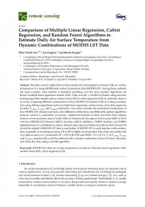
Figure 1. — Quantile regression function.
data, especially when compared to the parametric mean or average statistic. The QR model does not require the product characteristics or the response variable (IB in this study) to be normally distributed and does not have the other rigid assumptions associated with MLR. The first-order QR model has the form (Koenker 2005), Qyi具|x典 = 0 + ixi + F −1 u 共兲
R2k
is the coefficient of multiple determination for Xk where when regressed on the remaining p − 2 predictors in the model. High levels of multicollinearity (VIF > 10) can falsely inflate the least squares estimates; therefore, lower VIF values are desired (Kutner et al. 2004). Residual pattern analysis is key criteria for assessing model quality. Residuals should not have any pattern when plotted against Y, any X, or as a function of time. Heteroscedasticity is unequal variance of residuals and indicates that the model is ill-founded. Residual plots should not have any slope or bias with a E(i) = 0. SAS code for mixed stepwise regression. — When modeling manufacturing processes, it is important to consider the most recent data first, i.e., this data will be most informative for continuous improvement (Deming 1986, 1993). SAS code was used to develop the mixed stepwise regression MLR models for the four product types using the previously described Best Model Criteria. MLR models for all possible subsets were explored using the most recent data and then moving backward in time. Initial models were developed for the 50 most recent data records and additional models were developed for each additional record moving backward in time through the data. The aforementioned best model criteria were used in selecting the best model from the subsets provided by SAS. Quantile regression QR is intended to offer a comprehensive strategy for completing the regression picture (Koenker 2005). It is different from the MLR approach in that it takes into account the differences in behavior a characteristic may have at different levels of the response variable by weighting the central tendency measure. Also, this method uses the median as the measure of central tendency rather than the mean. The nonparametric median statistic may offer additional insight in the analysis of 42
[8]
where, Qyi is the conditional value of the response variable given in the ith trial, o is the intercept, i is a parameter, denotes the quantile (e.g., = 0.5 for the median), xi is the value of the independent variable in the ith trial, Fu is the common distribution function (e.g., normal, Weibull, lognormal, other, etc.) of the error given , E(F −1 u ()) = 0, for i = 1, . . . , n, e.g., F −1(0.5) is the median or the 0.5 quantile. Just as we can define the sample mean as the solution to the problem of minimizing a sum of squared residuals, we can define the median as the solution to the problem of minimizing a sum of absolute residuals (Koenker and Hallock 2001). The symmetry of the piecewise linear absolute value function implies that the minimization of the sum of absolute residuals must equate the number of positive and negative residuals, thus assuring that there were the same number of observations above and below the median (Koenker and Hallock 2001). Minimizing a sum of asymmetrically weighted absolute residuals yields the quantiles (Koenker and Hallock 2001). Solving n
min
兺 共 y − 兲,
i
[9]
i=1
where the function (.), e.g., in Eq. [9], is the tilted absolute value function appearing in Figure 1 that yields the th sample quantile as its solution (Koenker and Hallock 2001). To obtain an estimate of the conditional median function in quantile regression, we simply replace the scalar in Eq. [9] by the parametric function (xi, ) and set to 1/2.4 To obtain estimates 4
Variants of this idea were proposed in the mid-eighteenth century by Boscovich and subsequently investigated by Laplace and Edgeworth (Koenker and Hallock 2001).
APRIL 2008
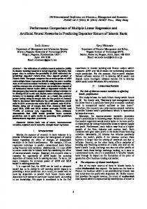
Figure 2. — Adjusted R2 for all possible subsets explored for 0.750-inch.
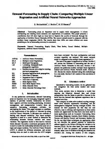
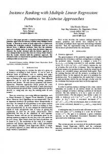
Figure 4. — Adjusted R2 for all possible subsets explored for 0.6875-inch.
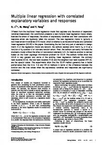
Figure 3. — Adjusted R2 for all possible subsets explored for 0.625-inch.
Figure 5. — Adjusted R2 for all possible subsets explored for 0.500-inch.
of the other conditional quantile functions, replace absolute values by (.), e.g., Eq. [9], and solve
parameters. The RMSE of the model was 7.69 psi and the maximum VIF for any independent variable was 5.03. Residual patterns for the MLR model were homogeneous (Table 1). Recall the RMSE estimates the SD of the residual error, which is the square root of the MSE which is the SSE divided by the degrees of freedom.
n
ˆ 共兲 = min
兺 共 y − 共x , 兲兲.
i
i
[10]
i=1
For any quantile ⑀ (0,1). The quantity ˆ () is called the th regression quantile.
Results and discussion The internal bonds of four different product types of MDF were analyzed. Each product type represents a different board thickness in inches (i.e., 0.750-inch, 0.625-inch, 0.6875-inch, and 0.500-inch). All possible subset MLR models were explored for the four product types using R2a as a key indicator for determining the best subset model (Figures 2, 3, 4, and 5). The R2a for all possible subsets was an indicator of a MDF manufacturer’s stability in reproducing product quality from one production run to the next, i.e., product types where the R2a changes slowly as more records were added moving back in time may indicate less volatility in IB between production runs, and also that changes in processes occur less frequently between production runs of the product type. Once acceptable MLR models were obtained (i.e., using the best model criteria), commonalities in the independent variables were explored among the four product types. Product types 0.750-inch and 0.625-inch For the 0.750-inch product type a MLR model was developed with an R2a of 75 percent, 50 degrees of freedom and 11 FOREST PRODUCTS JOURNAL
VOL. 58, NO. 4
For the 0.625-inch product type a MLR model was developed with an R2a of 72 percent, 53 degrees of freedom and 11 parameters. The RMSE of the model was 6.05 psi and the maximum VIF for any independent variable was 5.60. Residual patterns for the MLR model were homogeneous (Table 1). Common independent variables for the 0.750-inch and 0.625-inch MLR models were highlighted as bold in Table 1. “Refiner Resin Scavenger %” and “Core Water to Wood” were common for both 0.750-inch and 0.625-inch product types. It was surprising to see the scaled estimates for “Refiner Resin Scavenger %” differ in sign for each product type.5 The “Refiner Resin Scavenger %” has a negative scaled estimate of approximately −9.12 psi on IB for 0.750-inch while the “Refiner Resin Scavenger %” has a positive scaled estimate of approximately 8.40 psi on IB for 0.625-inch. This may indicate that “Refiner Resin Scavenger %” was an important
5
Scaled estimate is a helpful statistic in MLR models in that it illustrates the relative influence of independent variables on the response variable. The scaled estimate is the influence that an independent variable has on the response variable when the independent variable moves one-half its range used in the model.
43
Table 1. — MLR models for product types 0.750-inch and 0.625-inch.
product types that have varying throughput levels at the refiner. To examine the influence of “ReScaled Scaled finer Resin Scavenger %” beyond Parameters estimate p-value Parameters estimate p-value the mean effect on IB, QR was exFace MDF temperature −12.565