Comparison Between Multiple Linear Regression And Feed forward ...

International Journal of Applied Science and Technology

Vol. 1 No.4; July 2011

Comparison Between Multiple Linear Regression And Feed forward Back propagation Neural Network Models For Predicting PM10 Concentration Level Based On Gaseous And Meteorological Parameters Ahmad Zia Ul-Saufie (Corresponding author) Clean Air Research Group, School of Civil Engineering Engineering Campus, Universiti Sains Malaysia 14300 Nibong Tebal Pulau Pinang, MALAYSIA School of Civil Engineering Universiti Sains Malaysia Email: [email protected], Phone: + (60)4-5996227 Ahmad Shukri Yahya Nor Azam Ramli Hazrul Abdul Hamid Clean Air Research Group School of Civil Engineering, Engineering Campus Universiti Sains Malaysia, 14300 Nibong Tebal Pulau Pinang, MALAYSIA. ABSTRACT

Air pollution is a major issue that has been affecting human health, agricultural crops, forest and ecosystem. Local environmental or health agencies often need to make daily air pollution forecasts for public advisories and for input into decisions regarding abatement measures and air quality management. Forecasts are usually based on statistical relationships between weather conditions and ambient air pollution concentrations. Multiple linear regression models have been widely used for this purpose, and well-specified regressions can provide reasonable results. The aim of this study is to determine the best technique between Multiple Linear Regression (MLR) and Feedforward Backpropagation Artificial Neural Network (ANN) models for predicting concentration in Pulau Pinang. Multiple regression models and neural networks are examined for Seberang Jaya, Pulau Pinang with the same independent variables, enabling a comparative study of the two approaches. Model comparison statistics using Prediction Accuracy (PA), Coefficient of Determination (R2), Index of Agreement (IA) , Normalised Absolute Error (NAE) and Root Mean Square Error (RMSE) show that ANN is better than MLR.

Keywords: Particulate Matter (PM10), Multiple Linear Regressions, Artificial Neural Network, Ozone 1. INTRODUCTION

Particular matter is the term given to the tiny particles of solid or semi-solid material found in the atmosphere. PM10 is the fraction of particulates in air with aerodynamic diameter of less than or equal 10 micrometers. Sulaiman and Mohd Nor (2005) study in quarry area in Selangor had found significant health effect of PM10 to the quarry workers. The level of PM10 in that area was between 167μg/m3 and 278μg/m3. From 28 respondents aged below 55, 16 of the workers experienced bad health effects due to high PM 10 level such as chest pain (7 cases), breathing difficulty (3 cases), eye irritation (3 cases) and asthma (1 case). In addition, many previous researches discussed about the effect of PM10 to human health from minor effects to serious effects, increased hospital admission and premature death (Dockery and Pope, 1994; Griffin, 1994; Alley et al., 1998; Wark et al., 1981; Caselli et al., 2009). Regression techniques have a long history of use as forecasting tools in multiple disciplines. Regression models have the advantage of simple computation and easy implementation. Researchers have applied regression models for predicting PM10 concentration in different areas such as Municipality of Bari, Italy (Casseli et al., 2009), Athens in Greece (Grivas and Choloulakou, 2006), Mediterranean City, Greece (Papanastasiou et al., 2007) and Seberang Perai, Malaysia (Ghazali, 2006). Due to the nature of linear relationship in the parameters, regression models may not provide accurate predictions in some complex situations such as non-linear data and extreme values data. 42

© Centre for Promoting Ideas, USA

www.ijastnet.com

Regression model also have limitation such as the need to fulfill regression assumptions and multiple collinearity between independent and dependent variables causes regression model to be inefficient (Molazem et al., 2002; Zaefizadah et al., 2011). Artificial neural networks (ANN) are useful tools for prediction, function approximation and classification. It is well suited to extracting information from imprecise and non-linear data such as air quality and meteorology (Caselli et al., 2009). Extreme values are represented well if they are present in the data set that the network was trained on, but the network cannot accurately extrapolate values outside the training set. Besides that, various different networks can be used by determining the type and number of layers and control feedback. (Adielson, 2005). Currently, the applications of neural networks have become more popular for predicting PM10 concentration such as discussed by Chaloulakou et al., 2003; Chelani et al., 2003; Gardner and Dorling, 1998; Perez et al., 2000; Grivas and Chaloulakou, 2006; Caselli et al., 2009; Papanastasiou et al., 2007). Comparison between MLR and ANN methods have also been done (Chaloulakou et al., 2003; Gardner and Dorling, 1998; Papanastasiou et al., 2007). Short term forecasting of PM10 is needed for preventive and evasive action during air pollution. Local environmental or health agencies often need to make daily air pollution forecasts for public advisories and for input into decisions regarding abatement measures and air quality management. This paper discussed two methods for predicting PM10 concentration that are Multiple Linear Regression and Artificial Neural Network using feedforward backprogation method. 2. MATERIALS AND METHOD

2.1 Study area and local meteorology Pulau Pinang state is situated on the north-western coast of peninsula Malaysia. The area of Pulau Pinang state is 1046.3 km2, latitudes 5o 8’ - 5o 35’, longitude 100o 8’-100o 32’. Pulau Pinang State consists of two parts, Pulau Pinang Island and mainland Seberang Perai. The island has an area of 285 km2 and is connected to Seberang Perai by ferry and by the 13.5 km long Pulau Pinang Bridge. Pulau Pinang is a big town that experienced rapid development in industries along with economic sector. The growth of Pulau Pinang state as an urban-industrial centre has generated a number of problems. As a developing town, Pulau Pinang cannot avoid the occurrences of air pollution. This was proven when several unhealthy days were recorded (Department of Environment, Malaysia ; 2007). The development of industrial activities for the last 15 years represents another area of concern which is directly related to the present study. It has been estimated that both transport and industries produce about 99% of the major pollutant emissions in the study area (Ghazali, 2006). Based on Department of Environment (DoE) record, Seberang Perai, is one of the most polluted areas in Malaysia (Department of Environment, Malaysia; 2004), therefore, Seberang Perai was selected as the focus area of the research. 2.2. Air quality data Annual hourly observations for PM10 in Seberang Prai, Pulau Pinang, Malaysia from January 2004 to December 2007 were selected for predicting PM10 concentration level. The hourly observations was transformed into daily data by taking the average PM10 concentration level for each day. So 1430 observations were used for this research since the data for September 2007 were missing and were not included in the analysis. Table 1 shows the characteristic for the PM10 data and the chosen dependent variables for the monitoring site in Seberang Perai, Pulau Pinang. Table 1: Descriptive statistics for dependent and independent variables The chosen variables such as relative humidity (RH), wind speed (ws), nitrogen dioxide (NO2), temperature (T), carbon monoxide (CO), sulphur dioxide (SO2), ozone (O3) and previous day PM10,t-1 were selected to study the influence on PM10 concentration. Temperature was reported to have strongest effect on PM10 concentration (Md Yusoff et al., 2008). Particulate nitrates and sulphates formed from NOx and SOx were emission are major components of PM10 (Sawant et al., 2004; Kim et al., 2000). Godish (1997) found that horizontal winds play a significant role in the transport and dilution pollutant. A study in Birmingham, United Kingdom have shown that there is a positive relationship between wind speed and coarse particulates for the summer because of resuspension of soil particles (Harrison et al., 1997). Relative humidity describes the amount of water vapour that exists in a gaseous mixture or air and water in percentage. It can affect PM10 concentration when the values are greater than 55%. 2.3. Multiple Linear Regression Multiple linear regression is one of the modelling technique to investigate the relationship between a dependent variable and several independent variables. 43



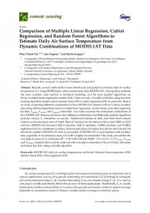
This is a generalisation of the simple linear regression model. In the multiple linear regression model, the error term denoted by 𝜀 is assumed to be normally distributed with mean 0 and variance 𝜎 2 (which is a constant). 𝜀 is also assumed to be uncorrelated. We assume that the multiple linear regression model have k independent variables and there are n observations. Thus the regression model can be written as (Kovac-Andric et al., 2009) (1) Yi   0   1 x1i  k x ki  i with i  1,, n . Where 𝑏𝑖 are the regression coefficients, 𝑥𝑖 are independent variables and 𝜀 is stochastic error associated with the regression. To estimate the value of the parameters, the least squares method was used. 2.4 Artificial Neural Network A feed-forward neural network with a back propagation learning algorithm was used due to its simplicity and widespread applications (Podner et al., 2002). Back propagation network was created by generalizing the Widrow-Holf learning rule to multiple-layer networks and non-linear differentiable transfer functions. Weights and biases are updated using a variety of gradient descent algorithms. The gradient is determined by propagating the computation backward from outputs layer to first hidden layer. If properly trained, the back propagation network is able to generalize to produce reasonable outputs on inputs it has never “seen” as long as the new inputs are similar to the training inputs. This research used two layer feed forward back propagation. The first hidden layer used the tangent sigmoid transfer and outputs layer or second layer with linear transfer function. The multiple layers of neurons with nonlinear differentiable transfer function allow the network to learn nonlinear and linear relationship between input and output vectors. An example of two layer feedforward back propagation network is shown in Figure 1. Figure 1: Feedforward Backpropagation network Mathematically, ANN model can be written as in equation (2) 𝑦 = 𝑓 𝑥, 𝜃 + 𝜀 (2) Where 𝜃 is the weights vector (parameters), x is the vector of independent variables that was used previously and 𝜀 is the random error component. Equation (3) is the unknown function for estimation and prediction from the available data: 𝑛 𝑌 = 𝑓 𝑣𝑜 + 𝑚 (3) 𝑗 =1 ℎ 𝜆𝑗 + 𝑖=1 𝑥𝑖 𝑤𝑖𝑗 𝑣𝑗 Where Yi = network output, f = output layer activation function, 𝑣0 = output bias, m = number of hidden units, h = hidden layer activation function, 𝜆𝑗 = hidden unit biases ( j = 1 , … , m), n = number of input units, 𝑥𝑖 = input vector ( i = 1 , … , n), 𝑤𝑖𝑗 = weight from input unit i and hidden unit j, 𝑣𝑗 =weights from hidden unit j to output ( j = 1 , … , m) 2.5 Performance Indicators Performance indicators were used to evaluate the goodness of fit for the MLR and ANN to determine which method is appropriate to represent the PM10 concentration in Seberang Prai, Pulau Pinang. Performance indicators are selected to determine the best method for predicting PM10 concentration are normalized absolute error (NAE), Root Mean Square Error (RMSE), index of agreement (IA), prediction accuracy (PA), and coefficient of determination (R2). The equations used were reported by Lu (2003). Table 2: Performance indicator 3. RESULTS AND DISCUSSION

The parallel development of multiple linear regression and neural network models were carried out to assess the predictive performance of the models. For this, the same inputs were used for the development and comparison of the two approaches. 3.1 Multiple Linear Regression Models Multiple linear regression models were developed with 1430 observations using SPSS (PASW) version 18.0. Hence the best model with the highest R2 (0.942) is obtained. The range of values for Variance Inflation Factor (VIF) for the independent variables is between 1.3 until 2.01. The value is lower than 10 indicating that there is no multicollinearity between the independent variables. Durbin Watson statistic shows that the model does not have any first order autocorrelation problem (DW=1.824).Therefore, the regression coefficients for the dependent variable were used to derive the equation for PM10 as given by equation (4). 44


www.ijastnet.com

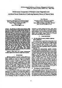
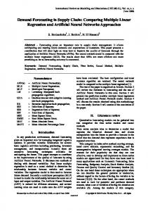
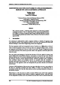
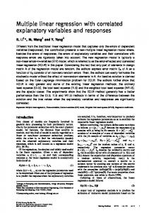
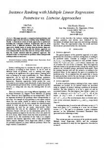
PM10 = -92.748 + 0.655 PM10,t-1 + 0.245ws + 0.104RH + 944.491NO2 + 2.682T + 944.491CO + 496.734SO2 + 58.532O3. (4) The study of residuals (or error) is very important in deciding the adequacy of the statistical model. If the error shows any kind of pattern, then it is considered that the model is not taking care for all the systematic information. Figure 2a indicates histograms of the residuals of PM10 model. The residual analysis shows that the residuals are distributed normally with zero mean and constant variance. The plots of fitted values with residuals for PM 10 model are shown in Figure 2b indicating that the residuals are uncorrelated i.e. the residuals are contained in a horizontal band and hence obviously that variance are constant. Figure 2:(a) Standardized residual analysis of PM10, (b) Correlations of fitted values with residuals for PM10 The multiple correlation coefficients (R) for MLR model is 0.942 with p-value less than 0.001, which is significant at 1% level of significance. Figure 3(a) show the plots of predicted and measured values of PM10. Figure 3: Correlation between measured and predicted values of PM10 by using (a) MLR and (b) ANN 3.2. Artificial Neural Network Models A 3-layer neural network with two hidden layers were developed with selected variables, namely relative humidity (RH), wind speed (ws), nitrogen dioxide (NO2), temperature (T), carbon monoxide (CO), sulphur dioxide (SO2), ozone (O3) and previous day PM10,t-1 as input and PM10 as output neurons. Out of 1430 observations, 1100 data were used for training and 330 for validation. It was split up using the duplex algorithm. The optimum number of epochs was determined by examining the training error and validation error for the selected algorithm. Figure 4 shows the graph of prediction and observed value of PM10 using ANN models. The multiple correlation coefficients (R) for ANN model is 0.946, which is significant at 1% level of significance (pvalue less than 0.001). Figure 3(b) show the plots of predicted and measured values of PM10 using ANN. Figure 4: Prediction and observed value of PM10 using ANN models 3.3. Comparison between MLR and ANN Comparing MLR and ANN for PM10 concentration prediction in Seberang Perai, Pulau Pinang, the performance indicators were used to measure the accuracy of predicted value. Table 3 shows the performance indicator values. The values of the accuracy measure namely Prediction Accuracy, Coefficient of Determination, Index of Agreement have value greater than 0.8 indicating that the predicted values are highly accurate. However, the accuracy measures for ANN is better than for MLR. The value for the coefficient of determination is 0.887 which is greater than 0.8, it showed MLR can still be use for predicting PM10 concentration. The values of the error measures namely Normalised Absolute Error and Root Mean Square Error are smaller for ANN than for MLR. This shows ANN give the better result than MLR based on accuracy measures and error measures. So, ANN should provide a better prediction than MLR. Table 3: Performance Indicator between MLR and ANN models 4. CONCLUSION

The aim of this study was to compare a Multiple Linear Regression model and Feedforwad Backpropagation ANN for predicting PM10 concentration in Seberang Perai, Pulau Pinang. Relative humidity (RH), wind speed (ws), nitrogen dioxide (NO2), temperature (T), carbon monoxide (CO), sulphur dioxide (SO2), ozone (O3) and previous day PM10,t-1 were used as independent variables. The quality and reliability of the developed models were evaluated via performance indicators (NAE, RMSE, PA, IA and R2). Assessment of model performance indicated that neural network can predict particulate matter better than multiple regressions. Similar conclusions were found by previous studies (Chaloulakou et al., 2003; Gardner and Dorling, 1998; Papanastasiou et al., 2007). However models adequacy checked by various statistical methods showed that the developed multiple regression models can also be used for prediction of PM10. Acknowledgement: This study was funded by Universiti Sains Malaysia under Grant 304\PAWAM\\6039013304. Thank you to Universiti Sains Malaysia and Fellowship Scheme for providing financial support to carry out this study and also thanks to the Department of Environment Malaysia for their support. 45



5. REFERENCES Alley R. E. and Associates, Inc., (1998). Air Quality Control Handbook. United States of America: McGraw-Hill Companies Adielson S., (2005). Statistical and neural networks analysis of pesticide losses to surface water in small agricultural catchments in Sweden. M.Sc Thesis, Sweden University, Sweden. Chaloulakou, A., G. Grivas and N. Spyrellis, (2003). Neural network and multiple regression models for PM 10 prediction in Anthens: A comparative assessment. J. Air and Waste Manage. Assoc., 53: 1183-1190. Chelani, A. B., Gajghate, D. G., Hasan, M. Z. (2003). Prediction of ambient PM 10 and toxic metals using artiﬁcial neural networks. J. Air and Waste Manage. Assoc., 52(7), 805–810. Caselli, M., Trizio, L., de Gennaro, G., Ielpo, P. (2009): A simple feedforward neural network for the PM 10 forecasting: comparison with a radial basis function network and a multivariate linear regression model. Water Air Soil Pollution. 201, 365–377. Department of Environment, Malaysia (2004). Malaysia Environmental Quality Report 2004. Kuala Lumpur: Department of Environment, Ministry of Sciences, Technology and the Environment, Malaysia. Department of Environment, Malaysia (2007). Malaysia Environmental Quality Report 2007. Kuala Lumpur: Department of Environment, Ministry of Sciences, Technology and the Environment, Malaysia. Dockery, D.W. and Pope, C.A. III, (1994). Acute Respiratory Effects of Particulate Air Pollution. Journal. Annual Revision Public Health 1999. Volume 15, pp. 107-132. Fitri N.F, Ghazali N. A, Ramli N.A, Yahaya A.S, Sansudin N., Madhoun W.A (2008), Correlation of PM 10 concentration and weather parameters in conjuction with haze event in Seberang Perai, Pulau Pinang, Simposium Kebangsaan Sains Matematik ke 15, UTM, Malaysia. Gardner, M.W. and Dorling, S.R. (1998), Artificial neural networks (the multilayer perceptron) – a review of applications in the atmospheric sciences, Atmospheric Environment 32. (14/15), pp. 2627–2636. Godish, T. (1997) Air Quality (Third Edition). New York: Lewis Publishers. Griffin, D. R. (1994) Principles of Air Quality Management. Florida: CRC Press. Ghazali N.A. (2006) A Study To Assess The Effect Of Weather Parameters In Influencing The Air Quality In Malaysia. M.Sc Dissertation, Universiti Sains Malaysia, Malaysia. Grivas G. and Chaloulakou A. (2006), Artificial neural network models for prediction of PM 10 hourly concentrations, in the greater area of Athens, Greece, Atmospheric Environment, 40 , pp. 1216–1229. Kim B.M, Teffera S., and Zeldin M.D (2000), Characterization of PM2.5 and PM10 in the South Coast Air Basin of Southern California: part1-Spatial variation, J. Air and Waste Manage. Assoc., 50(12), 2034-2044. Kovac-Andric, E., Brana, J., Gvozdic V., 2009. Impact of meteorological dactors on ozone concentrations modeled by btime series and multivariate statistical methods. Ecol. Inf 4, 117-122 Lu, H. C. (2003) Estimating the Emission Source Reduction of PM10 in Central Taiwan. J. of Chemosphere. 54, p. 805-814. Harrison R.M., Deacon A.R., Jones M.R. and Appleby R.S. (1997), Sources and processes affecting concentrations of PM 10 and PM2.5 particulate matter in Birmingham (UK). Atmospheric Environment 31 (1997), pp. 4103–4117 Molazem, D., Valizadeh M. and Zaefizadeh M., (2002), North West of gentic diversity of wheat. J. Agricultural Sciences., 20; 353-431 Papanastasiou, D., Melas D., and Kioutsioukis I. (2007), Development and Assessment of Neural Network and Multiple Regression Models in Order to Predict PM10 Levels in a Medium-sized Mediterranean City. Water, Air, & Soil Pollution,. 182(1): p. 325-334. Perez P., Trier A. and Reyes J. (2000), Prediction of PM2.5 concentrations several hours in advance using neural networks in Santiago, Chile, Atmospheric Environment 34, pp. 1189–1196. Podnar, D., D. Koracin and A. Panorska, 2002. Application of artificial neural networks to modeling the transport and dispersion of tracers in complex terrain. Atmospheric Environment, 36: 561-570. Sawant A. A., Na. K., Zhu X.N., and Cocker D.R.(2004), Chemical characterization of outdoor PM2.5 and gas-phase compounds in Mira Loma, California, Atmospheric Environment .38(33),5517-5528. Sulaiman, N. and Mohd Nor, S.A. (2005) Zarahan terampai (PM 10) dan pengurusannya di kawasan kuari Semenyih, Selangor. In Jahi, J. M., Ariffin, K., Awwang, A., Aiyub, K., and Razman, M. R., (eds) Prosiding Seminar Kebangsaan Pengurusan Persekitaran 2005, UKM, Bangi, 2005, July 4-5 The Mathworks (2006), Applying Neural Netwok with MATLAB, Activemedia Innovation Sdn Bhd. Wark K., Warner C. F., Davis W. T. (1981) Air Pollution: Its Origin and Control, Second Edition. New York: Harper & Row, Publishers. Zaefizadah M., Khayatnezhad M., and Ghlaomin M., (2011), Comparison of Multiple Linear Regression (MLR) and Artificial Neural Network (ANN) in Predicting the Yield Using its Components in the Hulless Barley, J. Agriculture and Environmental Sciences., 10(1), 60-64.

46


www.ijastnet.com

6. TABLES AND FIGURES Table 1: Descriptive statistics for dependent and independent variables Variables PM10 (mg/m3) Ozone (ppm) Wind Speed (km/hr) Relative Humidity (%) T (oC) SO2 (ppm) NO2 (ppm) CO (ppm)

P

Mean

Median

Mode

Std. Deviation

Skewness

Kurtosis

Min

Max

67.241

57.875

109.896

29.517

0.914

0.840

21.167

222.792

0.017

0.017

0.011

0.007

0.438

0.311

0.002

0.053

6.523

6.4417

5.446

1.094

0.695

1.050

3.900

12.329

75.350

75.333

69.579

6.740

-0.086

-0.027

51.375

95.750

28.183

28.226

27.829

1.273

-0.318

-0.006

23.729

32.546

0.006

0.005

0.004

0.005

1.721

4.503

0.000

0.043

0.013

0.013

0.013

0.003

0.250

-0.001

0.003

5.025

0.496

0.4726

0.491

0.178

1.079

2.659

0.096

1.744

a1

IW1,1

s1 x1

n Rx1 1

a2 = y 2,1

b1 S1

1 s1x1

LW 2 x S1

n2 2 x1

b2 2x1

2x1

Figure 1: Feedforward Backpropagation network (The Mathworks, 2006)

47



Table 2: Performance indicator (Lu, 2003) Performance indicator Mean absolute error (MAE)

Equation

 P O

MAE  Normalized (NAE)

absolute

error

i

i 1

i

n NAE value closer to zero indicates better method.

n

NAE 

 Abs ( P  O ) i

i 1

i

n

O i 1

Index of agreement

Description MAE value closer to zero indicates better method

n

i

n  P  Oi 2   i 1 IA 1   n    Pi  O  O i  O  i 1



Prediction accuracy

 P

i

O 

 O

O 

n

PA 

i 1 n

i 1

Coefficient of determination (R2)

i

   2   

IA value closer to 1 indicates better method.



PA value closer to 1 indicates better method

2

2

 n    Pi  P Oi  O    i 1  R2   n.S pred .S obs    

2

R2 value closer to 1 indicates better method

Where; n

= Total number of annual measurements of a particular site.

Pi

= Predicted values of one set annual monitoring record

Oi

= Observed values of one set annual monitoring record

P

= Mean of the predicted values of one set annual monitoring record

O S pred

= Mean of the observed values of one set annual monitoring record

S obs

= Standard deviation of the predicted values of one set annual

monitoring record.

= Standard deviation of the observed values of one set annual monitoring record between input and outputs vectors.

(a) (b) Figure 2:(a) Standardized residual analysis of PM10, (b) Correlations of fitted values with residuals for PM1 48


www.ijastnet.com

(a) (b) Figure 3: Correlation between measured and predicted values of PM10 (mg/m3) by using (a) MLR and (b) ANN 220 Obs Pred 200

PM10(mg/m3)

180

160

140

Number of days

120

100

80

60

40

20

0

50

100

150

200

250

300

350

Figure 4: Prediction and observed value of PM10 using ANN models Table 3: Performance Indicator between MLR models and ANN models Performance Indicator Normalised Absolute Error Prediction Accuracy Coefficient of Determination Root Mean Square Error Index of Agreement

MLR 0.109 0.941 0.887 9.938 0.969

ANN 0.098 0.954 0.894 8.369 0.976

49