the new estimator will be unbiased and will have variance less than the variance of. Y alone. ... vector of 1's. The resulting minimum variance estimator has. V ar.
POSTER { Control, Navigation, and Planning: Theoretical analysis.
A Control Variable Perspective for the Optimal Combination of Truncated Corrected Returns Michael O. Du�
Department of Computer Science University of Massachusetts Amherst, MA 01003 du�@cs.umass.edu
Abstract This paper details further development of an idea rst suggested in (Barto & Du�, 1994)|that of bringing variance reduction techniques to bear upon the problem of optimally combining corrected truncated returns.
1 INTRODUCTION Consider a system whose dynamics are described by a nite state Markov chain with transition matrix P , and suppose that at each time step, in addition to making a transition from state xt = i to xt+1 = j with probability pij , the system produces a randomly determined reward, rt+1, whose expected value is R(i). The evaluation functionP, V , maps states to their expected, in nite-horizon discounted returns: t V (i) = E f 1 t=0 rt+1 jx0 = ig ; 0 < < 1. It is well known that V uniquely sati es a linear system of equations decribing local consistency: V = R + PV: One way (Watkins, 1989) of viewing the TD(�) algorithm (Sutton, 1988) is that it updates its current value function estimate V~ (xt) in the direction of a weighted combination of the following (in nite) family of estimators: (1) X [k] = rt + rt+1 + � � � k?1rt+k?1 + k V~ (xt+k ) k = 1; 2; ::::
| | | | |
1e+00
| | | | | | | | |
1e-01
|
Summed Squared Error
Weight
| |
|
|
|
0.25
|
|
0.50
Successive approximation 2 weights 3 weights 5 weights
| | | | |
|
0.75
1e+01
|
1.00
| |
| | | | | |
1e-02
| |
| 2
| | | | | | | | 3 4 5 6 7 8 9 10 Corrected Truncated Return Term
Figure 1: TD(�) weight sets.
1e-03 | 0
|
| 1
|
|
0.00 | 0
| 1
| 2
| 3
| 4
| 5
| 6
| | 7 8 Iteration
Figure 2: Convergence results.
For large values of k (such that k is small), the truncated corrected return, X [k] , is approxmately equal to the sampled discounted return, which is an unbiased estimate for V (xt ), and has variance equal to the variance of accumulated discounted rewards encountered along sample paths. For smaller values of k, the portion of total variance due to the variance of summed, discounted rewards beyond time horizon k is replaced by the variance of V~ (xtk ). If the approximate value function is equal to the true value function, then the variance of this \tail" will be less than the variance of the tail of sampled returns; if the approximate value function is in error, then in general X [k] will be a biased estimator. P [k ] In TD(�), the estimators X [k] are combined via Xw = 1 k=1 wk X ; where wk = (k ?1) ( new ) ( old � (1 ? �), and V~ (xt) is updated via V~ (xt) = (1 ? �)V~ ) (xt) + �Xw . The weighting function, wk , for the combination of truncated corrected returns is illustrated in Figure 1. For small values of �, the resulting estimate Xw is more heavily weighted toward X [k] 's with small values of k, estimators with potentially small variance but high bias. Watkins has suggested that a reasonable strategy might be to apply TD(�) with � near one at the outset of learning, so as to avoid the ill-e�ects of using biased V~ 's, then as con dence in the V~ 's grows, to slowly reduce � to reduce variance. The decaying exponential form of the weighting function gives rise to an update rule that can be implemented incrementally, but there is no reason to presume that the \best" combination of estimators would be weighted in this way for any value of �, in fact one might well suspect that the best weighting scheme would (at least) vary with state and time. In (Barto & Du�, 1994), it was suggested that the estimators X [k] could be interpreted as what are known as \control variables" in the literature of Monte Carlo variance reduction techniques. A control variable (Lavenberg & Welch, 1981) for a random variable Y , whose expected value, �, we are trying to estimate, is another random variable, C , that is correlated with Y and whose expected value is known or known to be the same as Y 0 s. A new estimator for � can be constructed that is a linear combination of Y and C , and if the combining is done in the right way, then the new estimator will be unbiased and will have variance less than the variance of Y alone. This paper investigates the consequences of applying a multivariable form of this
variance reduction technique to the problem of estimating a value function. In this setting, the control variables are the current estimate, V~ , together with the truncated corrected returns, X [k] . Admittedly, the algorithms suggested by the full-blown control-variable approach, even when realizable, are computationally intensive, but the real goal of this analysis is to gain increased insight into temporal di�erence methods and, in particular, to improve upon heuristic schemes like the one o�ered by Watkins for introducing or \scheduling" bias|the e�orts summarized in this paper seek more sophisticated methods based upon a rigorous theory.
2 A MINIMUM VARIANCE APPROACH Consider the (in nite) family of estimators, (1), for V (xt), together with X [0] = V~ (xt ). If the V~ (�) are unbiased, then so are the X [k] , and the unbiased linearly P1 [k ] weighted combination of the X , k=0 wk X [k] , having minimum variance is obtained by choosing 1 ?1 w� = 1�0�X?111 (2) X |where �X denotes the covariance matrix of the estimators X [k] and 1 is a column vector of 1's. The resulting minimum variance estimator has (
1 X
)
V ar wk� X [k] = w�0 �X w� = 0 1?1 : 1 �X 1 k=0
(3)
With regard to the covariance matrix �X , consider a generic entry: [�X ]m;n
= Cov(X m] ; X [n] ) = Cov [
! nX ?1 k n k m ~ ~
rt+k + V (xt+m ); rt+k + V (xt+n ) : k=0 k=0
mX ?1
Without loss of generality, suppose that m � n, and let � � = rt rt+1 � � � rt+n?1 V~ (xt+m ) V~ (xt+n ) : Z 0 def Then � � X [m] = 1 2 � � � m?1 0 � � � 0 m 0 Z = Cm0 Z � � X [n] = 1 2 � � � m?1 m � � � n?1 0 n Z = Cn0 Z: But Cov(Cm0 Z; Cn0 Z ) = Cm0 �Z Cn, where �Z is the covariance matrix associated with Z . One can now address the (less messy) problem of computing, estimating, or approximating entries in �Z . Generic entries are of the form (1) Cov(rt+i ; rt+j ), (2) Cov(rt+i ; V~ (xt+m )) or Cov(rt+i ; V~ (xt+n )), and (3) Cov(V~ (xt+m ); V~ (xt+n )). 1 This (Gauss-Markov) formula for w� may be derived by,
for example, to solve the constrained optimization problem: n?Pusing Lagrange multipliers �2 o P 1 [k ] ? V (xt ) , subject to k wk = 1. minw E k =0 wk X
Supposing for the moment that w� could be computed, the new estimate for V (xt ) P1 (1) is simply V~ (xt) = k=0 wk� X [k] . Optimally weighted estimates could be constructed for the other states as well, and for each state the variance of the corresponding new V~ (1) decreases in a well-de ned way given by Equation 3. The variance (covariance) structure of the improved V~ (1) , in turn, enters into the calculation of the next iteration of optimal weight calculations through the generic entries of type (2) and (3) in �Z listed in the previous paragraph. Conceptually, the result of following this procedure is that each state will be assigned a distinct set of weights that change value in an \open loop" fashion as value-function updates occur. The weight prescription is the \best" in the sense of expected dynamics and updates over an entire ensemble of simulations whose initial estimates are unbiased and have an initial covariance matrix speci ed by �V . One straightforward way of obtaining initial unbiased value function estimates, V~ (0) , would be to simply use the sample mean (computed from one or more trials) of accumulated discounted rewards along sample paths of length k starting from each state, where k is chosen to be large enough to ensure that k is small. Using one long sample path to construct such estimates for more than one state necessarily implies some degree of correlation between the intial set of V~ 's. (0)
3 FULL BACKUP CASE If the expected rewards, R, and transition matrix, P , are known, then one can consider the following family P of (\fullyPbacked up") estimators for V (xt): with xt ?1 i N (P i ) R(j )+ k PN (P k ) V~ (j ); k = assumed to be state I , X [k] = ki=0 Ij Ij j =1 j =1 0; 1; 2; :::; |where N denotes the number of states. It can be shown, using the same methods as in the previous section, that generic entries in the covariance matrix �X are given by
Cov(X [m] ; X [n] ) = m+n
N X
k=1
(P m )Ik
N X j =1
(P n)Ij Cov(V~ (k); V~ (j ));
(4)
and the covariance matrix associated with the new set of estimates has entries
Cov(VI ; VJ ) = (1)
(1)
N X
m=1
(
1 X
wkI k (P k )Im
!
k=0 the kth optimal weight
N X
n=1
Cov(V (m); V (n))
1 X
wkJ k (P k )Jn k=0 (5)
for state I . |where wkI denotes Example: Figure 2 plots summed-squared error versus iteration (average results over 25 trials of initial estimates having standard normal errors) for the full back-up version of the iterative Gauss-Markov algorithm with estimator sets of size 2,3, and 5. 2 applied to a ten-state problem with = :7. As expected, as the number of 2 For example, for an estimator set of size 2, fX [0]; X [1] g, taking m = 0 and n = 1 in
Equation 4 leads to �
P
�
V ar(V~ (I ))
Nj=1 (P P )Ij Cov(V~ (I ); V~ (j )) PN PN �X = 2
j=1 (P )Ij Cov(V~ (I ); V~ (j )) k=1 (P )Ik Nj=1 (P )Ij Cov(V~ (k); V~ (j )) ;
!)
estimators increases, so does the rate of convergence. As k ! 1, X [k] becomes the Neumann series for V , and the corresponding wk dominates the other weights. Similarly, for the case of two estimators (Equation 6), the optimal weights (optimal �) place more emphasis on X [1] (in fact, it is not unusual for X [0] to have negative weight 3 ). The following analysis further explains why an optimal weighting with an associated value of � > 1 should not be surprising. Equation 6 may be re-written as V (k+1) = [� P + (1 ? �)I ] V (k) +�R; and the xed point, V � , satis es this equation identically. Subtracting it from both sides yields an equation for the error: �(n+1) = [|� P +{z(1 ? �)I}] �(k): If e is an eigenvector for M�
P with eigenvalue �, then e is also a eigenvector for M� with eigenvalue �� = �� + (1 ? �): (7) The behavior of the error is governed by the eigenvalue of M� having largest magnitude. By setting the magnitudes of the values of �min and �max under the mapping de ned by (7) equal to one another, one arrives at the optimal choice of �� = 2? (1?2 �min ) (see Figure 3).
4 SAMPLE-BASED METHODS Can the sample-based approach of Section 2 be made to work in way similar to the model-based approach of the last section? One could construct sample covariance matrices, �^ X , in the usual way, but computational experience strongly suggests that using a sample covariance matrix, which has some amount of sampling variance (error), in \optimal" weight calculations does not work well. And unfortunately, analytical approaches must contend with the problem of calculating the covariance between mixtures rather than simple random variables; i.e., V ar(V (xt+1)) is not P the same thing as j Pxt;j V ar(V (j )). Suppose that R and P are unknown, but that the process has been observed as it evolves and accumulates rewards and that this information has been recorded in the following matrix and vector: 2
P^
6 = 664
n11 nn211 n2
.. . n
N1
nN
n12 nn221 n2
.. . n
N2
nN
��� ��� ��� ���
n1N nn21N n2
.. . n
NN
2 Pn1
3
i=1 ri (1) 7 6 Pn2n1 6 i=1 ri (2) 7 7 6
3 7 7 7 5
R^ = 66
n2
.
. 6 4 PnN. r
i=1 i (N ) nN
nN
7 7 7 5
(8)
and the rule for updating entries in the covariance matrix �V is just the Equation 5 with \1" replaced by \1" in the summations over k. These expressions, along with Equation 2, in essence specify how � should change in the TD(0)-type update rule: "
V
(k +1)
(I ) = (1 ? �)V (I ) + � R(I ) + (k )
N X
#
PIj V (j ) (k )
j =1 3
R. Sutton & S. Singh have communicated similar empirical results.
(6)
Stochastic Approximation (known structure)
α =1 1 γ
α =2
1
1/ γ
Stochastic Approximation −−TD(0)
No Model
SOR with Iterative optimal Gauss−Markov (sample covariance) relaxation
Stochastic Approximation (accelerated)
1
Prioritized Sweeping
Max Lhood (rank−1 update)
SOR (with P−estimate)
Figure 3: Geometry of optimal �.
Full Model
Iterative Gauss−Markov
Iterative with P−estimate
Figure 4: The model/no-model \continuum."
|where N is the number of states, nij is the number of i ! j transitions observed, ni is the total number of transitions from state i observed, and ri(k) denotes the ith sample of reward observed in transit from state k. These are the maximum-liklihood estimates of P and R given the observed data, and one may derive con dence intervals for P^ and R^ as well (Nanthi & Wassan, 1987) (Billingsley, 1961). Motivated by the preceding analysis of ideal values for �, consider the re(k +1) laxation recursion = h i with P and R replaced by their estimates: V ^ V � satis es Equation 6 identically, and subtracting (1 ? �)I + � P^ V (k) + �R: it from both sides results in an equation for the evolution of error: V (k+1) ? V � = [(1 ? �)I + � P ] (V (k) ? V � ) + �(�R + �P V^ (k)), where �R = R^ ? R and �P = P^ ? P are asymptotically normal. The error equation may be approximated by �(k+1) = I�(k) + ( P ? I )��(k) + �w, where w is vector of normal, mean-zero noise. This is a disrete-time, stochastic, bilinear system (Mohler, 1980) that we would like to drive to zero as quickly as possible (through choice of �), and there exist advanced methods for doing so (e.g., Gutman, 1981). A simple method, based on simply minimizing the expected squared error at the next step, suggests choosing �(k+1) = � (I ? P^�) ((II ??
PP^^))��+P � , where �i is the ith component of the mean zero i i noise, which should decay to 0 as P^ and R^ converge. 0
0
0
2
5 Discussion: TD-relaxation with Models and Approximate Models With regard to the full backup version of the TD(0)-type recursion, Equation 6, it was shown in a Section 3 that, under certain assumptions, the � yielding fastest convergence to a xed point has a value greater than one; i.e., that the relaxation should be over-relaxed. On the other hand, if we have no knowlege of the transition matrix P , the usual TD(0) scheme (which is a form of stochastic approximation), having observed a transition from state i to j , in essence takes P to be a matrix of all zeroes but for a single value of one in the i; j th position (i.e., it uses an instantaneously sampled version of the true model), and prescribes a choice of � that is severely under-relaxed. This suggests that there is a continuous spectrum of
optimal choices for �|that the best � depends on the degree of con dence one has in the \model," P . Figure 4 views TD(0) as lying at the extreme no-model end of the spectrum. At the opposite end of the spectrum, methods choose their step-sizes in an optimal (minimum variance) fashion based on full knowledge of system parameters. In between these two extremes lie a mixture of methods including those based on constrained models (e.g., stochastic approximation acceleration) and estimated models (e.g., incremental maximum liklihood). The \incremental maximum liklihood algorithm" works as follows: Suppose that, after having observed a number of transitions, P^ (and R^ ) estimates have been constructed as in Equation 8, (I ? P^ )?1 has been computed, and that we now observe a transition from state i to state j . The i ! j transition changes only the ith row of P^ , and the corresponding change in (I ? P^new )?1 can be computed without starting from scratch by making use of the following well-known \rank-one update" Theorem: Let A be a matrix with inverse N = A?1. Let h be a column vector and ? 1 � a row vector. Then N = (A ? h ) exists i� Nh 6= 1 and, if so, )( N ) N� = N + (1Nh ? Nh : Let h be a column vector of all zeros but for a \1" in the ith position, and = ? ni (ni +1) [ ni1 ni2 � � � nij ? ni � � � niN ] : Then th ^ ?1 ^ ?1 (I ? P^new )?1 = (I ? P^old )?1 + [i columnth of (I ? Pold ) ][ (^I ? ? P1 old ) ] : 1 ? [i entry of (I ? Pold ) ] This formula gives rise to an online update rule for (I ? P )?1 that takes approximately N 2 operations per observation. The update gives the exact inverse. Gauss-Seidel takes number-of-contractions �N 2 per observation, where number-ofcontractions depends on the accuracy desired and is usually small but may occasionally spike to > N operations. Prioritized Sweeping (Moore, 1993) makes use of maximum liklihood estimates (8) as well and empirically outperforms Gauss-Seidel. It could be argued that the rank-one update algorithm is relatively straightforward to understand/implement; there are no parameters like Moore's � or , and convergence analysis is straightforward since it is directly coupled to the convergence of P^ and R^ to the true system parameters. Some nal comments regarding Figure 4: Since the early 1950's when Stochastic Approximation was rst introduced, there have been a number of schemes proposed for accelerating convergence. Among them, (Kesten, 1958) suggests maintaining step size at nomimal values until a change in sign of successive estimates occurs; (Jacobs, 1988) is recent related work. (Venter, 1967)'s method accelerates the rate of convergence by, in e�ect, estimating the slope of the underlying regression function at the desired root. More recently, (Dupuis & Simha, 1991) have suggested taking multiple samples at given operating points to reduce variance. Apart from these acceleration schemes for improving the standard algorithm, it should be noted that stochastic approximation is a rather general method for computing roots of
noisy (nonlinear) regression functions. In the case of the value-estimation problem, however, the sought-after value occurs at the intersection of a collection of linear manifolds| the standard algorithm could be improved upon by exploiting this fact (in Venter's method, for example, each data point contributes information about the slope of the regression function at its root).
Acknowledgements Thanks to Andy Barto and to the members of the Adaptive Networks Laboratory. This work was supported in part by the National Science Foundation under Grant ECS-9214866 to Professor Barto.
References A. Barto & M. O. Du� (1994). Monte Carlo Matrix Inversion and Reinforcement Learning. In D. S. Touretzky (ed.), Advances in Neural Information Processing Systems 5. San Mateo, CA: Morgan Kaufmann. P. Billingsley (1961). Statistical Inference for Markov Processes Univerity of Chicago Press. P. Dupuis & R. Simha (1991). On sampling controlled stochastic approximation. IEEE-TAC 36:915-924. P. Gutman (1981). Stabilizing Controllers for Bilinear Systems. IEEE-TAC 26(4), pp. 917-922. R. Jacobs (1988). Increased Rates of Convergence Through Learning Rate Adaptation. Neural Networks 1:295-307. H. Kesten (1958). Accelerated Stochastic Approximation. Ann. Math. Statist. 29:41-59. S. Lavenberg & P. Welch (1981). A perspective on the use of Control Variables to increase the e�ciency of Monte-Carlo simulations. Management Science 27:322-335. R. Mohler & W. Kolodzki (1980). An Overview of Stochastic Bilinear Control Systems. IEEE-TAC pp. 917-922. A. Moore & C. Atkeson (1993). Prioritized Sweeping: Reinforcement Learning with Less Data. Machine Learning 13:103-130. K. Nanthi & M. Wassan (1987). Statistical Estimation for Stochastic Processes, Queen's Papers in Pure and Applied Mathematics, no. 78. R. Sutton (1988). Learning to Predict by the Method of Temporal Di�erences. Machine Learning 3:9-44. J. Venter (1967). An Extension of the Robbins-Monro procedure. Ann. Math. Statist. 38:181-190. C. Watkins (1989). Learning from Delayed Rewards. PhD Thesis Cambridge University.