Proceedings of the American Control Conference Anchorage, AK May 8-10,2002
Adaptive Speedh'osition Control of Induction Motor with Unknown Load Torque Hou-Ran Lee,' Li-Chen F d s 2and Su-Hau Hsu'
' Department of Electrical Engineering Department of Computer Science and Information Engineering National Taiwan University, Taipei, Taiwan, R.O.C. E-mail:
[email protected]
Abstract The paper proposes an adaptive speedposition
nowadays. Not only the power drive is particularly
tracking control of an induction motor subject to unknown
considered [2] but also the power issue joint with
load torque. The controller is developed based on a
performance is seriously taken into account [3]-[5].
dynamic model obtained from the d-q-axis model (w.r.t. the
In general applications, indirect vector control of
stationary reference frame) of the motor under a special
induction motor is widely applied, where the rotor flux is
nonlinear coordinate transform so that either speed or
estimated rather than being measured. This requires a
position control objective can be fulfilled. The underlying
priori knowledge of the machine parameters, which makes
design concepts is to endow the close-loop system with
the indirect vector control scheme machine dependent.
so-called maximal power transfer property while under lack
Given the fact that parameters may change significantly
of knowledge of some key system parameters, such as the
with temperature and there are some states which are not
rotor resistance, motor inertia and motor damping
easily acquired, design of appropriate observers becomes
coefficient. To be rigorous, the proposed control scheme
crucially important to the success of the control [6].
comes along with a thorough proof derived based on
Recently, the sensorless field oriented control scheme
Lyapunov stability theory. The experimental results are also
gradually appears as a popular control method for induction
given to validate the effectiveness of the presented control
motor [7]-[101. Taking the output (speed) feedback
scheme.
seemingly is another effective alternative dealing with the problem with unknown resistance [8]. On the other hand,
1. Introduction
the load torque structure is also a very important
The induction motor control is an important issue in both motion control and servo control applications, because the induction motor can operate in a wide-range of both
knowledge for controller design to
achieve high
performance control. Given
the
above
observation,
we
propose
a
torque and speed. And, their efficiency and robustness are
speedposition tracking control scheme based on the
useful features in industry.
indirect FOC with the property of maximal power transfer
The field oriented control (FOC) methodology is a
to the rotor. Moreover, the proposed control scheme
popular control scheme of induction motor to achieve the
handles the problems with both uncertainties of rotor
high performance operation [ 11. The control schemes based
resistance and load torque, respectively. The system
on indirect FOC are much more popular due to the
parameters of the induction motor, except its rotor
advantages in applications. On the other hand, the issue of
resistance, and mechanical parameters, are known as
power efficiency of induction motor is well concerned
mentioned previously. For rigorousness, the developed
0-7803-7298-0/02/$17.00 0 2002 AACC
4583
control scheme is thoroughly analyzed via Lyapunov
voltages in d-qframe of the voltagelfed induction motor are
stability theory, and the asymptotic convergence property is
defined as
soundly proved. The experimental results are given to
CV,
=
validate the performances.
J"-v' 'dr
'qr
CV,
=
-
(2)
+ 'dr
then the power transferred to the rotor of induction motor
2. Maximal Power Transfer of Induction Motor In this section, we will first review the mathematical description of the operational principle of an induction motor in the following subsection. After that, we will present some important results related to the underlying
is maximal subject to the constraint
(v: +vi)
= (V I C ) *
at any time [4][5][9].
Of course, V does not have to be a constant. Instead, it
concept to facilitate our subsequent controller development
offers one D.O.F. (Degree of freedom) control to the
As has been well known, the dynamical model of an
system, but normally it will converge to a constant (in
induction motor can be simplified by a d-q-axis coordinate
regulation problem) or is related to the desired output (in
transformation
tracking problem) when the system approaches to the
from
the
original
three
phase
representational frame to some rotational-reference frame.
steady state.
But
3. Preliminary
to
make
implementation
feasible,
the
stationary-reference frame is more popularly used. Thus,
To proceed with the controller design, we first introduce
here we adopt the following group of (d-q-axis)
the observers to estimate the unmeasurable rotor flux, and
coordinate-transformed
the unknown rotor resistance under the following
dynamical
equations
of
an
induction motor [ 1I]
assumption:
(A.2) All the states are measurable except the rotor flux. Parameters including rotor resistance, rotor inertia, damping coefficient, and the payload coefficient are assumed unknown. Due to Assumption (A.2), we have to build an observer and a parameter estimator to estimate the rotor flux as well as the rotor resistance. There exist various types of flux observers and parameter estimators in the literature, which have been described in [ll]. Here, in this paper we adopt
(1)
the observer and estimator design similar to those in [lo], where the states and the Parameters are defined as shown in
which is based on the stator current and rotor flux dynamics
the nomenclature.
as shown below:
Before we continue the control of position of the
=k,,6-(l,+4"Rr)iq5 +RriqrpZ+w,~*++cVp+uq7
induction motors, we first make a basic assumption as
L& =k& -&
shown below: (A. 1) The induction motor is assumed without saturation,
hysteresis, eddy currents, and spatial flux harmonics.
Proposition 1. Under the assumptions (A.I),
if the
input
4584
+&"e)& +RrAdr+ pLrwrAqr +bcV,
L , A ~=~- & I q r + PL,W,A~, +L+,,kriqJ Lradr= -&aa
- pLrwraq,+L,,,Rrids9
+ud
where k,, k , > 0.Let the auxiliary signals
uy
and
U,
vector
@
vector
w=
= [ J , ~ bo b,
b2]I’,and the known function
be
designed as follows:
‘
[’
w,
sgn(w,)
T
w, sgn(q)d . In the sequel,
we will assume that 0 is unknown, which together with the unknown constants
J,
and B, forms the set of
unknown parameters as has been mentioned in the former assumption (A.2). On the other hand, there exists a proper input signal V such that the steady state of the system exactly achieves the purpose of speed tracking, i.e., w, = U,, and the objective
o,j = - ( k o + k d , o , ) i ; , - - 5i~ - P w , q q ’
of maximal power transfer (Proposition 1). To this end, we
(4)
L,
first introduce a reasonable assumption as shown below:
with k,,, kq2, k,,, kd2 > o . Thus, the property of the
(A.3)
proposed observers is summarized in the following
dynamics shown in (1) by introducing a nonlinear state
proposition, whose proof can be found similar to that in
transformation given as shown in [ 5 ] . Under the
[lo].
transformation with Proposition 1, the dynamical equations
Proposition 2. If the dynamic equations of the induction
shown in (1) can then be transformed to the following
motor are described as system ( I ) with all the states being
dynamic model:
bounded and measurable except the rotorflux. Then, the
x2
=
A;,+Aj,
> 0, and then further simplify the
x, = -2a,x, +2a2x,+-2 k r , v
fi
flux observer and the rotor resistance estimator designed as in (3) can guarantee that
Aqr -)aq, , Ad, +Ak
and X2
kr -.+
R, as t +.m with the system being persistently
excited (PE), where all the auxiliary signals being defined
=
-2a,x2 +2a,x,
i3 = a+, + a,x;-
(a,+ a , ) ~ ,+ p x , ~ ,
in (4).
For general mechanical systems, the load torque is a function of the rotor speed w ,as
i4 = - px,x, JXS
T , = J , ~ + s g n ( w , ) b b + 4 ~ + 4 s g n ( w , ) ~=J&+ f,(W,) . This assumption is more realistic than a constant load torque. For example, it can be shown that bearings and many other viscous forces (including those encountered by cutting tools) vary linearly with speed, where the large-scale fluid systems such as pumps and fans have loads that typically vary with the square of the speed. Therefore, the mechanical load in the form aforementioned can be rearranged as T~= W,T@ with the constant parameter
- (a,+ a,)x, + &V
= asx4-fL(~S)’
where the parameters a,,a2,a3,a4,aS are defined in the nomenclature and the load structure f L ( x s ) is well defined in the previous subsection. Since controller design based on a particular system structure often involves complicated algorithms which may likely lead to high implementation cost, it is highly motivated that designing a controller that can be applicable to a vast class of system structure is quite preferable. 4. Design of SpeedPosition Controllers
4585
(5)
In order to prove the stability of system (5) with the following proposed controller, we first present the following useful working lemma.
1
+ a4)x4+ px3x5+ ~4~ - uses- Pze41
V = -[(a,
A
Lemma 1. Ifthe state variable xS = q ,its derivative is, and the stator currents iqs, id are all bounded, then the
I ^
x4d = -(bo+ bl xs a5
states x, ,i = 1..5 of system (5)are all bounded.
Proof: First, we restate the dynamic equation of
A
A
A .
+ b2 x i + J
md
- pie,)
7
x2
from system (5) as
4 =-b4x, +2a,x, =-204% +2a,(iqAq +ihAb)S+4x, +Go$
parameter estimators:
9
where the positive parameters aS,a,are defined in the nomenclature and is =s:i
+ j i . Thus,
x2 =
6 = -esrWT.
A,* = A:r + Ajr
is bounded provided is is bounded. Besides, from system
with W = [hdsmod(x5) x, smod(x5)x~1' 0 = [ J bo b, b2]',
(3,if
while all the intemal signals are kept bounded.
X,
and its derivative i5are bounded, then
bounded immediately.
Finally,
from
X,
is
[SI the states
Proof: Omitted here, referred to Ref.[9]. In order to design the position tracking controller, we
and x , , which are composed of bounded signals
X,
augment the system ( 5 ) with additional equation (6) as
is and A,,and hence all the states of system (5) are shown
shown follow:
Q.E.D.
to be bounded as well.
X6
Before we introduce the design of the controller, in order
where x,
= 0,
= xs
(6)
9
indicates the rotor position of the induction
to avoid dealing with the discontinuous function sgn(x), we
motor. To proceed with the design of the position controller,
approximate it y the so-called sigmoid function smod(x)
we first make an assumption as follow:
defined below:
(A.4) The desired position command
e, E c3 is three-time
differentiable smooth function with
e, ,e,, ,e, ,and e:
eYx - e-Yx
sgn(x) =smod(x)
9-=
eYx + e-Y'
being all bounded.
where y > 1 determines the slope of the function. By
Thus, if the desired speed command satisfies assumption
taking such approximation, we will be able to differentiate
(AS), then the position tracking controller can be designed
the payload function f , ( w , ) for the subsequent purpose of
as stated in the following theorem.
controller design.
Theorem 2. Consider the induction motor system (5) and
Theorem 1. Consider an induction motor whose dynamics
the Eq. ( 6 ) under the Assumptions (A.1). (A2), (A.4), and
are governed by system (4) with unknown load torque and
(AS). Ifthe speed command is defined as
rotor resistance under the assumptions (A.1) and (A.2). Given a trajectory
twice-diferentiable 0,with
md,hd and
smooth #d
desired
if
< e6,n e, - k,e6,"smod(e6), otherwise,
speed
are all bounded, then
ie6i
the following control input can achieve the control
with k, BO, Then, the rotor position tracking error
objective
e,
W,
mr + 0,
as t
asymptotically)
+m
with
(i.e. xs = m, will follow the
control
input
= x6
-e,
will converge to zero asymptotically with the
control input V being designed as in Theorem 1. And, all the internal signals are thus kept bounded.
4586
R, = 0.83!2, R , = 0.53R, L, = 0.08601H, L, = 0.08601H,
Proof:
L,,, = 0.08259H, 4 poles, rated current 8.6 A, 220 V, 60 Hz,
In order to prove the theorem completely, the proof is divided into two steps as shown below:
AC. J , and €3,
1) The speed command
The
U,
function with w d ,bd,and
is a twice-differential smooth &jd
2 ) To prove that the state
X,
X,
-
X,
load
J Lhr+ bosgn(w,) btu,
torque
is
TL
=
+b2sgn(w,)wf.In experiment, there
is no load applied on the induction motor. The control gains
the assumption (AS) and the design of speed command. By Theorem 1, all the internal states
mechanical
+
being all bounded due to
areassumedunknown.
are a,=IO,
are kept bounded.
is bounded and the rotor
0, =IO
k, = 0.01, k , = 200
with k,, = k,, = k,, = kq2 = 0.003, and of
the
observers
gains.
The
position tracking error e, converges to zero, we rearrange
experimental results of both speed and position tracking are
- 4, = e, +U, - 4,. If the error dynamic equation as i, = i6
demonstrated in the following cases.
we choose the Lyapunov function as
v, = l e : ,
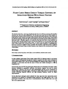
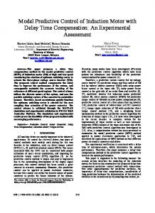
( 1 ) The experimental results of a benchmark speedposition
then the
2
v6 becomes
time derivative of
v6=(
command
if le,(
-k,ei + e,e,,
The speedposition command is like a sort of benchmark problem to validate the proposed controller. Figure 1 (or 2)
< e,,
shows the boundedness of estimated. parameters and also
-k,e,, le61+e,e,, otherwise,
the performances of the proposed controller with a where e, = X,
-ed,and
eS = X 5 - U d ’
benchmark speedposition command.
As our proposition, the upper bound of le,[ is e,,
.
+ e,e,
the experiments
are conducted
without the
information of the deviation of rotor resistance, the motor
Therefore, the time derivative V, I -kle:
All
inertia and the damping coefficient of the induction motor.
= -2k,V6 + e6es
9
And, the parameters of load torque are unknown, either. which readily implies boundedness of e, and, hence, the
6. Conclusion
e,(= x,) . Finally, the control objective:
In this paper, we first develop a special nonlinear
e, -+ 0 as r -+ w is apparently achieved provided the speed
coordinate transform which makes the rotor flux norm, the
-+ -. Moreover, as a result from step 1
electric torque and the rotor speed as individual variables
rotor position
error
eS -+0 as t
x2 ,
and step 2, the entire internal signals x i , i=1..6 are all
and xS , respectively. Then, we propose the
field-oriented Lyapunov-based controllers for an induction
QED.
bounded.
X,
motor to control the speed and position, respectively. And,
5. Experimental Results To validate the performances of the proposed controller,
they can also deal with both the uncertainty of rotor
we hold a series experiments with a 4-ploe, 3-phase
resistance and the unknown load torque. The experimental
squirrel-cage induction motor which rated power 3-HP with
results validate the performances mentioned above.
a
Reference
1000 pulsehev
encoder.
Detail
parameters
and
specification will be found in below. The software we adopt
[I] R. Marino, S. Peresada, and P. Tomei, ”Global Adaptive
the SimulinkTM 3.0 and MatlabTM 5.2, we use the
Output Feedback Control of Induction Motors with
Simu-DriveTM to combine motor control card with
Uncertain Rotor Resistance,” IEEE Trans. Automat. Contf,
SimulinkTM/RealTime WorkshopTM.Then we can directly
Vol. 44, NO. 5, pp. 968-983, 1999.
apply the simulation program to proceed experiments.
[2] S. K. Sul, and T. A. Lipo, “Design and Performance of a
4587
High-frequency Link Induction Motors Drive Operating at
NOMENCLATURE
Unity Power Factor,” IEEE Trans. Indust. Appl., Vol. 26, pp.
D =
434-440, 1990.
p
(LsLr-$)
a, = L,R,/D
= LmID
K, = 3pLm/2Lr
a, = L m R s / D a, = L,,R,/D
[3] G S. Kim, I. J. Ha, and M. S. KO, “Control of Induction Motors for Both High Dynamic Performance and High
a4 = L,R,ID
Power E ffiency,” IEEE Trans. Indust. electron., Vol.. 39,
L, = -R, L; Lm
NO.4, pp. 323-333, 1992.
a, = L , K , I D
L,
=
L o Lm
[4] H. T. Lee, L. C. Fu, and H. S. Huang, “Speed Tracking Control with Maximal Power Transfer of Induction Motor,” Proc. IEEE 3qh Con$
On Decision and Control,
pp.925-930,2000. [5] H. T. Lee, J. S Chang, and L. C. Fu, “Exponential Stable
1
’
I
“
I
7,
.
431 0
2
IOY
.
.
.
. ,
Nonlinear Control for Speed Regulation of Induction Motor I . Adap. Contr: & with Field Oriented PI-Controller,” Inr. .
Sign. Proc., Vol. 21, No.23, pp. 297-321,2000.
I
.
0
2
so1
.
‘ 4
I 8
PI =mid bl . .
I
8
.,
.
’
‘
‘
1
4
8
.
.
.
m=midm
1 I
[6] R. Krishnan, and A. S. Bharadwaj, “A Review of Parameter Sensitivity and Adaptation in Indirect Vector Controlled Induction Motor Drive Systems,” IEEE Trans.
.x
m
Power Electron., Vol. 6, No.4, pp. 434-440, 1990.
[7] M. Bodson, J. Chiasson, and R. T. Novatnak, “Nonlinear
Speed
Observer
for
Figure 1. Experimental results of speed tracking
High-Performance
Induction Motor Control,” IEEE Trans. Indust. Electron.,
Vol. 42, NO.4, pp. 434-440, 1995. [8] R. M. Mario, S . Peresada, and P. Valigi, “Output Feedback Control of Current-Fed Induction Motors with Uncertainty of rotor resistance,” IEEE Trans. Contr. Syst. Tech., Vol. 4, No. 4, pp. 336-347, 1996.
[9] H. T. Lee, and L. C. Fu, “Nonlinear Control of Induction Motor with Unknown Rotor Resistance and Load Adaptation,” Proc. American Control Conference, pp. 55-59,2001. [ 101 Y. C. Lin and L. C. Fu, “Nonlinear Sensorless Indirect
Adaptive Speed Control of Induction Motors with Unknown Rotor Resistance and Load”, Int. J. Adap. Contr: & Sign. Proc.. Vol. 21, No.23, 2000.
[ l l ] P. C. Krause, Analysis of Electric Machinery, McGraw-Hill, 1986.
4588
Figure 2. Experimental results of position tracking