A Feature Extraction Method Based on Stacked Auto-Encoder for Telecom Churn Prediction Ruiqi Li, Peng Wang, and Zonghai Chen ✉ (
)
Department of Automation, University of Science and Technology of China, Hefei, China
[email protected], {pwang,chenzh}@ustc.edu.cn
Abstract. Customer churn prediction is a key problem to customer relationship management systems of telecom operators. Efficient feature extraction method is crucial to telecom customer churn prediction. In this paper, stacked auto-encoder is introduced as a nonlinear feature extraction method, and a new hybrid feature extraction framework is proposed based on stacked auto-encoder and Fisher’s ratio analysis. The proposed method is evaluated on datasets provided by Orange, and experimental results verify that it is authentically able to enhance the perform‐ ance of prediction models both on AUC and computing efficiency. Keywords: Churn prediction · Feature extraction · Stacked auto-encoder
1
Introduction
Telecommunication industry depends heavily on customer base to maintain stable profits. Service providers nearly have no choice but paying more attention to retain customers. Therefore, an efficient customer relationship management system, especially a churner prediction model, is badly needed by telecommunication industry. Many factors influence the accuracy of churn prediction models. In general, a predic‐ tion model performs better if the original dataset contains more characteristic variables, which are also called features. However, too many characteristic variables usually bring about some other troubles e.g. over-fitting, or frequently require too large memory etc. In consequence, rebuilding characteristic variables in data preprocessing stage plays a significant role in the whole modeling process, which is named as feature extraction professionally. Several data mining technologies have been applied in churner prediction success‐ fully, including artificial neural networks [1] (ANNs), decision trees [2], Bayesian networks [3], logistic regression [4], Ada-Boosting [5], random forest [4], proportional hazard model [6] and SVMs. What’s more, abundant research achievements have been provided recently. Utku Yabas et al. [7] built an ensemble classifier consisting of a group of well performing meta-classifiers, demonstrating that the performance of churn predic‐ tion can be significantly improved. Bashar Al-Shboul et al. [8] investigated the appli‐ cation of a churn prediction approach by combining Fast Fuzzy C-Means (FFCM) and Genetic Programming (GP) for predicting possible churners, and proved promising capability in the field. However, studies that focus on feature extraction methods are relatively less. E.g. Yin Wu et al. [9] proposed a framework which was adaptable to © Springer Science+Business Media Singapore 2016 L. Zhang et al. (Eds.): AsiaSim 2016/SCS AutumnSim 2016, Part I, CCIS 643, pp. 568–576, 2016. DOI: 10.1007/978-981-10-2663-8_58
A Feature Extraction Method Based on Stacked Auto-Encoder
569
different data types and carried experiments out on a structured module to demonstrate the validity of the two-phase feature selection method. Wei-Chao Lin et al. [10] concluded that feature selection and data reduction in data preprocessing could produce better datasets to structure an optimal model, while the cost of training was observably decreased. Considering all the views above, we attempt to introduce the stacked auto-encoder (SAE), based on the deep learning theory, as a nonlinear feature extraction method for churn prediction, which is inspired by its successful application in computer vision. Furthermore, we propose another feature extraction framework named Hybrid Stacked Auto-Encoder (HSAE), which combines the SAE with Fisher’s ratio analysis. The proposed framework aims to extract intrinsic features of an original dataset and improve the performance of the telecom churn prediction model both on AUC and computing efficiency. We organize this paper into three main sections. In Sect. 2, we introduce two conventional feature extraction methods and the proposed method sequentially. In Sect. 3, experiments and tabulated results that demonstrate our contributions are exhibited. The paper is concluded in the final section in order to direct future studies.
2
Feature Extraction Methods and Criterions
In general, feature extraction methods are recognized as two types. One is to select the most effective part of features from the original high-dimensional features directly. The generated dataset is a subset of the original dataset practically. Suppose that the original dataset X contains N features, and a new datasets Y contains n features, then the expres‐ sion is:
X:{x1 , x2 , ⋯ , xN } → Y:{y1 , y2 , ⋯ , yn } yi ∈ N, i = 1, 2, ⋯ , n;n < N
(1)
The other one is to project the original features from high-dimensional space to lowdimensional space. The generated dataset is a map of original dataset. Suppose that the original dataset X contains N features, and a new dataset Y contains M features, then the expression is:
X:{x1 , x2 , ⋯ , xN } → Y:{y1 , y2 , ⋯ , yM } (y1 , y2 , ⋯ , yM ) = f (x1 , x2 , ⋯ , xN )
(2)
Among various feature extraction methods, Fisher’s ratio analysis is a representative method belongs to the first type, and principal component analysis (PCA) is a repre‐ sentative method belongs to the second type. What’s more, the introduced SAE belongs to the second type as well and the proposed hybrid framework aims to combine both advantages of the two types.
570
R. Li et al.
2.1 Fisher’s Ratio Analysis Fisher’s ratio analysis [11], which is also called Fisher linear discriminant, is an efficient approach for feature extraction in statistical pattern recognition. Suppose that there exist two types of label points in a k-dimension data space, and each dimension denotes a feature component. For a certain feature, once the square of the difference between means of each class is bigger and the sum of variances of each class is smaller, then the feature has better discriminability. Formally, it can be formulated as follow:
J(Fk ) =
(𝜇1 − 𝜇2 )2 𝜎12 + 𝜎22
,
(3)
in which 𝜇i , 𝜎i2 (i = 1, 2) are respectively the mean and variance of the ith class. The above idea is to estimate Fisher’s ratio for every feature in the original dataset, and select the ones with top scores in feature selection phase. 2.2 Principal Component Analysis PCA [12] is a linear feature extraction method, which performs by transforming the data into a low-dimensional linear subspace. Mathematically, a workflow for the PCA includes following steps. • Step 1: Figure out the sample mean of the original dataset 𝜒=
1 ∑o x o i=1 i
1 ∑o • Step 2: Compute the covariance matrix C = (x − 𝜒) ⋅ (xi − 𝜒)T o i=1 i • Step 3: Calculate the eigenvalues 𝜆1 , ⋯ , 𝜆l with the corresponding eigenvector h1 , ⋯ , hl of the matrix C, and arrange the eigenvalues in descending order. • Step 4: Record the transformation matrix as H T = [h1 , h2 , ⋯ , hl ]T , and the projected matrix is S = [s1 , s2 , ⋯ , so ]T = XH T .
Only the first several eigenvectors ranked in descending order of the eigenvalues are used, so that the number of selected principal components is decreased, and features are extracted simultaneously. 2.3 Stacked Auto-Encoder To avoid the potential (nonlinear) information loss caused by Fisher’s ratio analysis and PCA, we introduce SAE [13] as a new technique to be applied in telecom churn predic‐ tion field, which can be treated as a nonlinear feature extraction method based on the deep learning theory. Generally, SAE is a feedforward neural network with an odd number of hidden layers, which is shown schematically in Fig. 1. The whole neural network is designed to minimize the mean squared error between the output and the input layer. Conceptu‐ ally, it is trained to recreate the input and to compress the original data in the hidden
A Feature Extraction Method Based on Stacked Auto-Encoder
571
layer, while preserve as much intrinsic features as possible. When data point xi is used as input, the new representation yi, which is usually projected to a space of lower dimen‐ sionality, can be acquired by extracting node values in the middle hidden layer. Math‐ ematically, details for pre-training the SAE module are described as follows. Encoder
Input Data X
Output Data X
Low-dimensional Representation Y
Decoder
Fig. 1. Schematic structure of a SAE
SAE [14] is a deep network constituted with autoencoding neural networks in each layer. In the single-layer case, corresponding to an input vector x ∈ ℝn, the activation of each neuron, hi , i = 1, ⋯ , m is computed by
h(x) = f (W1 x + b1 ),
(4)
where h(x) ∈ ℝm is the pattern of neuron activations, W1 ∈ ℝm×n is the weight matrix, b1 ∈ ℝm is the bias vector, and sigmoid activation function is generally used to allow the auto-encoder learning a nonlinear mapping between the low-dimensional and highdimensional data representation. Output of the network is formulated by x̂ = f (W2 h(x) + b2 ),
(5)
where x̂ ∈ ℝn is the pattern of output values, W2 ∈ ℝn×m is a weight matrix, and b2 ∈ ℝn is a bias vector. Once a set of p input vectors x(i) , i = 1, ⋯ , p is given, the weight matrices W1 and W2 are calculated by back-propagation and gradient descent methods to minimize the reconstruction error
e(𝐱) =
∑p i=1
||x(i) − x̂ (i) ||2 .
(6)
In the multi-layer case, we train up the network layers in a greedy layer-wise approach successively. The first layer receives training samples with original features as input. After its reconstruction error achieves acceptable levels, a second layer is added,
572
R. Li et al.
then a third layer, etc. Furthermore, fine-tuning can be executed once we obtain the train labels 𝐲 ∈ ℝ for supervised learning. 2.4 Hybrid Stacked Auto-Encoder In order to take both advantages of the two feature extraction types, we propose a new feature extraction framework named hybrid stacked auto-encoder. The framework is described in Table 1. Table 1. HSAE algorithm for feature extraction
2.5 Classification and Criterions Criterions can hardly be carried out directly on the extracted features. It is common to set a criterion function to combine feature extraction methods with subsequent classi‐ fication algorithms. The classifier employed in the experiment is Logistic Regression. Mathematically, it can be formulated as a task of finding a minimizer of a convex function f (𝐰) =
T 1 ∑n 𝜆 log(1 + e−y𝐰 𝐱 ), ||𝐰||22 + i=1 2 n
(7)
the vectors xi ∈ ℝd are the training data examples, and yi ∈ ℝ are their corresponding labels. The fixed parameter 𝜆 ≥ 0 for L2-regularization defines the trade-off between the two goals of minimizing the loss and the model complexity.
A Feature Extraction Method Based on Stacked Auto-Encoder
573
For telecom churn prediction, the algorithm outputs a binary logistic regression model eventually. Given a new data point, denoted by x, the model makes prediction by applying the logistic (sigmoid) function f (𝐰T 𝐱) =
1 , 1 + e−𝐰T 𝐱
(8)
and outputs a probability value for each class. Therefore, there is a prediction threshold, e.g. t, which determines what the predicted class will be. If f (𝐰T 𝐱) > t, the outcome is positive, or negative otherwise. Tuning the prediction threshold will change the precision and recall of the model. So we use the receiver operating characteristics [15] (ROC) graph as the criterion. The area under the ROC curve, abbreviated as AUC, has an important property in statistics: the AUC of a classifier equals to the probability that the classifier ranks a randomly chosen positive instance higher than a randomly chosen negative instance. As a result, we regard the classifier with higher AUC as the better choice, and the embedded feature extraction method as the better choice as well.
3
Experiments and Discussions
The raw dataset for our experiments is gathered from KDD website based on marketing databases from the French telecom company Orange. The standard desktop computing platform is equipped with dual core 3.20 GHz processor and a RAM of 8 Gb. The experiment is conducted with Scala based on Spark machine learning library and Matlab toolbox for dimensionality reduction. 3.1 Dataset and Initial Preprocessing The raw dataset has 50,000 examples with 230 original features, including 190 numeric features and 40 categorical features. It’s impossible to use domain expertise because the data were encrypted and feature names were hidden [7]. Variables are polluted by large numbers of missing values. Worse still, most of the variables are in different dynamic ranges. Therefore, initial preprocessing and feature extraction play crucial roles. The initial preprocessing includes handing of missing values, discretization of the numeric features, aggregating of the categorical values, encoding prepared variables and removal of redundant features. First, we remove the features with more than 95 % missing values. Then, missing values in numeric features are replaced with the mean, while add additional features coding for the presence of each missing value correspond‐ ingly. Missing values in categorical features are tagged as “missing”, which are treated as new values. After that, numeric features are discretized into 6 new categorical features equably, which will be encoded together with other categorical features through onehot encoders. If a categorical feature has more than 10 distinct values, then we keep the 9 most frequent categories and group the rest in a category called “Others”. After removing the original numeric features and other redundant features, we finally obtain 496 features with binary value “0” or “1” simply.
574
R. Li et al.
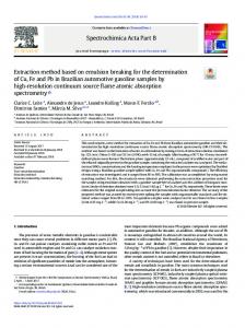
Furthermore, if we regard each feature as a pixel, which is a basic conception in computer vision field, then every data sample can be treated as a 31*16 grayscale image, which is shown in Fig. 2. We denominate the image as “customer’s informationportrayal” tentatively. The 50,000 examples with 496 features are then used as the material for feature extraction stage.
(a) A positive sample
(b) A negative sample
Fig. 2. Customer’s information-portrayals
3.2 Feature Extraction A series of experiments are designed to compare conventional feature extraction methods with the new proposed method. They are principally divided into 4 groups as follows: • • • •
Group 1: Extract features with PCA Group 2: Extract features with Fisher’s ratio Group 3: Extract features with SAE Group 4: Extract features with HSAE
50, 40, 30 and 20 features are extracted respectively for classification in each group. In details, the SAEs in group 3 and group 4 are designed with 7 layers without the output and input layer. To be highlighted, the first hidden layer is designed to be expanded to compensate for the representational capacity of sigmoid functions used in each layer, on the fact that neuron activations which transformed through the sigmoid function can’t represent as much information and variance as real-valued data. 3.3 Results and Discussions There still exists another two steps before classification. One is over-sampling. Copy the whole positive instances 13 times as the simplest over-sampling approach. The ratio of the positive and negative instances then equals to 1:1 approximately. The other step is data partition for cross-validation. The dataset is split into 2 subsets and the ratio of the training and testing sets equals to 7:3.
A Feature Extraction Method Based on Stacked Auto-Encoder
575
The AUC values of each experimental group are arranged and tabulated as follows. From Table 2 we conclude that a single SAE performs better than PCA, and it is approximately the same as Fisher’s ratio analysis. Moreover, the average runtime of SAE is about 2 h while the average runtime of Fisher’s ratio analysis is over 7 h. Furthermore, the proposed method in group 4 is verified to be better both in AUC and computing efficiency, which shortens the average runtime by 3.5 h comparing to group 2. Table 2. AUC of each experimental group PCA Fisher’s Ratio SAE HSAE
4
50 Features 0.6871 0.6972 0.6964 0.6989
40 Features 0.6839 0.6914 0.6937 0.6942
30 Features 0.6696 0.6914 0.6909 0.6925
20 Features 0.6656 0.6848 0.6893 0.6903
Conclusion and Future Works
In this paper, we introduce SAE to extract features in telecom churn prediction, which is compared with two types of conventional feature extraction methods. A new HSAE framework to accomplish the same task is also proposed. The experimental results demonstrate the efficiency of the proposed method. As the new conception of “customer’s information-portrayal” is proposed above, we will attempt to employ other deep learning algorithms, such as deep belief networks, convolutional neural networks etc., to deal with the telecom churn prediction problems, or even employ these algorithms to deal with other binary classification problems in the future.
References 1. Tsai, C.F., Lu, Y.H.: Customer churn prediction by hybrid neural networks. J. Expert Syst. Appl. 36, 12547–12553 (2009) 2. Qi, J., Zhang, L., Liu, Y., et al.: ADTreesLogit model for customer churn prediction. J. Ann. Oper. Res. 168, 247–265 (2009) 3. Kisioglu, P., Topcu, Y.I.: Applying bayesian belief network approach to customer churn analysis: a case study on the telecom industry of Turkey. J. Expert Syst. Appl. 38, 7151–7157 (2011) 4. Burez, J., Van den Poel, D.: CRM at a pay-TV company: using analytical models to reduce customer attrition by targeted marketing for subscription services. J. Expert Syst. with Appl. 32, 277–288 (2007) 5. Glady, N., Baesens, B., Croux, C.: Modeling churn using customer lifetime value. J. Eur. J. Oper. Res. 197, 402–411 (2009) 6. Van den Poel, D., Lariviere, B.: Customer attrition analysis for financial services using proportional hazard models. J. Eur. J. Oper. Res. 157, 196–217 (2004)
576
R. Li et al.
7. Yabas, U., Cankaya, H.C.: Churn prediction in subscriber management for mobile and wireless communications services. In: 2013 IEEE Globecom Workshops, pp. 991–995. IEEE Press, New York (2013) 8. Al-Shboul, B., Faris, H., Ghatasheh, N.: Initializing genetic programming using fuzzy clustering and its application in churn prediction in the telecom industry. J. Malays. J. Comput. Sci. 28, 213–220 (2015) 9. Wu, Y., Qi, J., Wang C.: The study on feature selection in customer churn prediction modeling. In: 2009 IEEE Systems, Man and Cybernetics, pp. 3205–3210. IEEE Press, New York (2009) 10. Lin, W.C., Tsai, C.F., Ke, S.W.: Dimensionality and data reduction in telecom churn prediction. J. Kybernetes 43, 737–749 (2014) 11. Wang, S., Li, D., Song, X., et al.: A feature selection method based on improved fisher’s discriminant ratio for text sentiment classification. J. Expert Syst. Appl. 38, 8696–8702 (2011) 12. Zhang, M., Li, G., Gong, J., et al.: Predicting configuration performance of modular product family using principal component analysis and support vector machine. J. J. Cent. South Univ. 21, 2701–2711 (2014) 13. Van der MLJP PEO, van den HH J.: Dimensionality reduction: A comparative review. In: Tilburg, Netherlands: Tilburg Centre for Creative Computing, Tilburg University, Technical report. 2009-005(2009) 14. Goodfellow, I., Lee, H., Le, Q.V., et al.: Measuring invariances in deep networks. In: Advances in neural information processing systems, pp. 646–654 (2009) 15. Fawcett, T.: An introduction to ROC analysis. J. Pattern Recogn. Lett. 27, 861–874 (2006)