A Fixed-Size Fragment Approach to Graph Mining M. Gholami∗1 and M. Norouzi†2 1
Department of Computer Engineering, West Tehran Branch, Islamic Azad University, Tehran, Iran. 2 Department of Applied Mathematics, School of Mathematical Sciences, University of Guilan, Rasht, Iran. July 19, 2014 Communicated by S.A. Edalatpanah Abstract Many practical computing problems concern large graphs. Some examples include the Web graphs, various social networks and molecular datasets. The scale of these graphs introduces challenges to their efficient processing. One of the main issues in such problems is that most of the mentioned datasets cannot be fit in the memory. In this paper, we present a new data fragment framework for graph mining. The original dataset is divided into a fixed number of fragments, associated with the number of the graphs in each dataset. Then each fragment is mined individually using a well-known graph mining algorithm (i.e. FSG or gSpan) and the results are combined to generate global results. A major problem in fragmenting graphs is concerning on similarity or dissimilarity of them. Another problem corresponds to the completeness of the output which will be discussed in this paper.
Keywords: graph mining, frequent subgraph, graph fragmentation, fixed-size fragment.
1
Introduction
Graph-based data mining or graph mining is defined as the extraction of novel and useful knowledge from a graph representation of data. In recent years, graph mining has become a popular area of research due to its numerous applications in a wide variety of practical fields. One of the most important concepts in graph mining is to find a frequent subgraph, i.e. to find a graph that is repeated in the main graph. Frequent subgraph mining delivers effective structured information such as common protein structures and shared patterns in object recognition. Recently numerous mining ∗ †
[email protected] [email protected]
25
International Journal of Mathematical Engineering and Science (IJMES) Volume 3 Issue 2 (February 2014) ISSN : 2277-6982 http://www.ijmes.com/ algorithms have been proposed to efficiently discover frequent subgraphs from the graph datasets. It is important to note that most of the existing algorithms employ memory-based approaches [1]. As a result, they face the scalability challenge when the input graph dataset cannot be held in the main memory. Since almost all graph mining algorithms assume that the dataset can fit into the main memory [2], mining these graph datasets remains a challenging computational problem. Several well-known graph mining algorithms are FSG1 [3], gSpan2 [4] and Gaston3 [5]. A comparative analysis and classification of these algorithms could be found in [6]. As discussed, many large graph datasets cannot load into memory. For example in a database consisting of 422 confirmed active compounds from AIDS antiviral screen database, only FSG, gSpan and Gaston can perform mining. When aiming the whole AIDS antiviral screen database, which contains 42689 compounds, only gSpan and Gaston can accomplish mining. Finally, for the whole NCI database which contains all 250,251 compounds, none of the above mentioned algorithms can process substructure mining on PCs, except when Gaston is running on SMP servers [7]. To address this challenge, some pre-processing techniques like graph partitioning algorithms have been proposed. These methods help to reduce the size of the input graphs. Two of the simplest techniques are the skipping and sequential fragments [8]. PartMiner algorithm [2] divides a large graph by cutting some edges to generate smaller units. Incremental clustering method [1] divides dataset based on dissimilarity of graphs and mines each partition individually. The goal of this study is to present a fragmentation technique to assign graphs to different fragments based on maximum dissimilarity. Then each fragment is mined individually using FSG and the results are combined to reach final frequent subgraphs. Comparing similar works, we propose a formula for the number of fragments. Also we employ FSG to mine each fragment, which employs the BFS search strategy [6]. Using more dissimilarity for assigning graphs to fragments, leads to a smaller number of frequent subgraphs in each fragment and consequently a larger number of certain subgraphs are discovered compared to the incremental clustering method and sequential fragments. In addition, we do not use intersections of frequent subgraphs of fragments which leads to smaller number of subgraphs requiring a second scan. The paper is organized as follows. Section 2 describes the primary concepts in graph mining. In section 3, we review other related works in graph mining and graph partitioning algorithms. Our method is presented in section 4. In this section we describe the idea of using dissimilarity inside each fragment and the method of combining local results to generate global results. In addition, we present two lemmas to prove the completeness of the results. Finally, the experimental results are reported in section 5. The results are compared with the incremental clustering method and sequential fragments. 1
Frequent Sub-Graph discovery Graph-based Substructure PAtterN 3 GrAph, Sequence and Tree extractiON 2
26
International Journal of Mathematical Engineering and Science (IJMES) Volume 3 Issue 2 (February 2014) ISSN : 2277-6982 http://www.ijmes.com/
2
Preliminary Concepts
A labeled graph is represented as a 4-tuple G=(V, E, α, β), where V is a set of vertices and E ⊆ V×V is a set of edges representing connections between all or some of the vertices in V. α: V → L is a mapping that assigns labels to the vertices, and β: V×V → L is a mapping that assigns labels to the edges. Given two labeled graphs G1 and G2 , G1 is a subgraph of G2 , if V(G1 ) ⊆ V(G2 ) and E(G1 ) ⊆ E(G2 ). In this case, G2 is called the supergraph of G1 . Given a graph dataset D, and a set of tuple (gid, G) where gid is the graph G’s identifier, the support of the graph G is the number of graphs in D that are supergraph of G. The problem of mining frequent subgraph is to discover the complete set of subgraphs in D, which their support is no less than the given minimum support.
3
Related Works
In recent years, various mining algorithms have been proposed to efficiently find frequent subgraphs from the graph datasets. AGM [9] proposed by Inokuchi et al. in 2000 and FSG [3] proposed by Kuramochi in 2001 are the most famous Apriori based approaches. These approaches mine the complete set of frequent subgraphs and generate numerous candidates during the mining process. Yan et al. proposed gSpan [4] in 2002 and Gaston [5] was proposed by Nijssen et al. in 2004 that employs pattern-growth based approaches. These methods are essentially memory-based and their efficiencies decrease dramatically when the graph database becomes large. A comparative analysis is offered in [6]. A number of data partitioning approaches were performed in order to achieve scalability [10–13]. These methods involve splitting a dataset into subsets, learning/mining from the subsets, and finally combining the results. According to the memory limitations inherent to the above mentioned algorithms for mining large graphs, partitioning methods have been utilized during the past years. PartMiner was introduced by Wang et al. [2]. This method discovers the frequent subgraphs by dividing the database by cutting some edges in-to smaller and more manageable units. Then, Gaston is employed to mine each unit. Nguyen et al. [8] introduced a horizontal partition approach which was extended by the same authors in 2008 [1]. In this method the original dataset is divided into partitions based on dissimilarity of graphs and each partition is mined individually using the gSpan. Then the results of each partition are combined to generate the global results.
4
The Fixed-size Fragment Method
Given a dataset D which includes graphs G1 to Gn , the main approach of our proposed technique is fragmenting D into a fixed number of partitions to provide the capability of loading each fragment in the memory individually. Initially the following questions must be addressed: • How many fragments are required? • Each graph Gi belongs to which fragment? 27
International Journal of Mathematical Engineering and Science (IJMES) Volume 3 Issue 2 (February 2014) ISSN : 2277-6982 http://www.ijmes.com/ • How can the results from fragments be combined to produce global results? In the remainder of this section, we first introduce and utilize our proposed method called the ”fixed-size fragment algorithm” to fragment the dataset and then we employ gSpan to mine the fragments. Finally, the obtained results using our technique are compared to the method mentioned in [8].
4.1
The Number of Fragments
The first step in fragmenting a dataset is choosing the number of fragments. A large number of fragments, i.e. smaller fragments, would generate innumerous frequent subgraphs in each fragment. Next step is to check these discovered subgraphs to investigate if they are frequent in the whole dataset. Thus generating a large amount of frequent subgraphs in each fragment is not recommended and would cause computational overhead. Additionally we should select an appropriate number of fragments which should allow loading the fragmented dataset into the memory. As a result, the number of fragments should maintain a proper balance in order to control the number of frequent subgraphs in each fragment and at the same time, consider the memory limitations of the platform. To the best of our knowledge, no formula for the proper number of fragments has been proposed in any of the previous related works. In our method the following formula is used to select the number of fragments:
k = [log(m)]
(1)
In which, m is the number of graphs in dataset and k is the number of fragments. The first step after finding k, is assigning graphs to them.
4.2
Assigning graphs based on Similarity or Dissimilarity
Supposing that we have k fragments, we assign the first k graphs to the k fragments. Then inside each fragment we define a characteristic parameter which is a set of the following parameters: • Number of edges of each graph, ei • Number of vertices of each graph, vi • One-edged subgraphs, Ii Consequently, the next k graphs are assigned to each fragment according to their maximum dissimilarity to the characteristic of that fragment. It is critical to mention that the characteristic of each fragment must be updated when a new graph is assigned to it. In our method we select maximum dissimilarity for assigning each graph, because dissimilar graphs inside a fragment will produce smaller number of local frequent subgraphs (the frequent subgraphs inside each fragment). Dissimilarity function between a graph and the ith fragment is denoted as follow:
28
International Journal of Mathematical Engineering and Science (IJMES) Volume 3 Issue 2 (February 2014) ISSN : 2277-6982 http://www.ijmes.com/ Algorithm1: GraphDisimilarity() Input: Ii , ei , vi and new graph G. Output: sumi , e gi , v gi . Begin 1. Let N be the set of 1-edge subgraphs in G. 2. e n = number of edges in G, v n = number of vertex in G. 3. S = N ∩X Ii . 4. sumi = (number of iteration of each member in S ) 5. e gi = number of iteration of e n in ei 6. v gi = number of iteration of v n in vi Assigning graphs to the suitable fragment is as follows: Algorithm2: GraphAssign() Input: Dataset D. Output: fragmented dataset Begin 1. n d = number of graphs in D. 2. Calculate number of fragments, namely k using Equation 1. 3. Assign first k graphs to the k fragments and calculate Ii , ei , vi for each fragment. 4. Assign next graph to the fragment that has minimum sumi using GraphDisimilarity(). 5. In the case of equal sumi , assign to the fragment that has minimum v gi or e gi . 6. Update Ii , ei , vi for each fragment. 7. The sizes of fragments are controlled to keep the balance between fragments. 8. Repeat step 4 to 7 until all graphs in the dataset are fragmented. Choosing a smaller number of local frequent subgraphs would reduce the computational space which is further discussed in the next section.
4.3
Frequent Subgraphs in Fragments
After determining the number of fragments, we assign each graph to a fragment and mine each fragment using gSpan to find the frequent subgraphs in each one of them. Then all frequent subgraps are listed in the set L(Fi ) (local frequent subgraphs of the ith fragment). In this work we are interested to find the frequent subgraphs in dataset D which we call them global frequent subgraphs. By taking union of all L(Fi ) we will construct a set of all the possible frequent subgraphs in D, denote as P. This union is quite different than a typical union in mathematics. In a regular union, iterative itemsets are listed in the union results only once. However, in our technique each frequent subgraph is listed in P as many times as it occurs in the union of all
29
International Journal of Mathematical Engineering and Science (IJMES) Volume 3 Issue 2 (February 2014) ISSN : 2277-6982 http://www.ijmes.com/ L(Fi )s. Items of P are called global candidates and are a candidate for being a frequent subgraph in D. The items in P with a frequency equal to or greater than the support are certainly frequent in D. We denote these items as C which is a part of the global frequent subgraphs. In the second phase, we only check the items of P-C in each fragment for the second time and calculate the support of each item. The summarization of our algorithm is given below:
Algorithm3: FixFragment() Input: Dataset D, minSup Output: frequent subgraphs Begin 1. Fragment dataset by using GraphAssign(). 2. Apply the gSpan subroutine with minSup to find the local frequent subgraphs for each fragment to get L(Fi ). 3. Compute the union of all L(Fi ), P: = ∪ L(Fi ). 4. For each item in P, if its iteration number ≥ minSup then assign it to C. //This means it is already frequent in D. 5. Check the items of P-C in each fragment for the second time to calculate the support of them. 6. Items not less than Support are returned.
4.4
Completeness of the results
The following lemmas guarantee the completeness of the mentioned algorithm. Lemma1. If g is a frequent itemset in database D, which is partitioned into k fragments F1 , F2 , ..., Fk , then g must be a frequent itemset in at least one of the k fragments. Lemma2. If database D is partitioned into k+1 fragments F1 , F2 , ..., Fk , then the number of Global candidates, denoted |Pk+1 |, is always greater than or equal to number of global frequent itemsets. Proof of these lemmas could be found in [14].
5
Experimental Results
In this section we apply our method to two real datasets. The first dataset, Chemical 340, is a Predictive Toxicology database containing 340 molecules which is equivalent that it has 340 graphs. This dataset is sparse. The second dataset, Compound 422, is a confirmed active compound from AIDS antiviral screen and contains 422 graphs and is dense. Using Equation 1 each dataset is divided into two fragments. Then by using the procedures mentioned in algorithm 2, graphs are assigned to the fragments. Each fragment is mined using gSpan algorithm to find local frequent subgraphs. The results are then combined using the routine discussed in algorithm 3 to find the global frequent subgraphs. We compare the results of our method with the sequential clustering
30
International Journal of Mathematical Engineering and Science (IJMES) Volume 3 Issue 2 (February 2014) ISSN : 2277-6982 http://www.ijmes.com/ and incremental clustering using supports 0.2 and 0.1. Table 1, provides a summary of applying the three methods to the molecule Chemical 340. Employing minSup 0.2 this molecule has 190 frequent subgraphs. For two fragments, in the sequential method, we find 223 frequent subgraphs in the first fragment and 291 frequent subgraphs in the second. In this case, after calculating P, 71 subgraphs are certainly frequent and 372 subgraphs must be checked again. Tables 1 and 2 display the improvement in our technique comparing to sequential and incremental clustering methods. We compare certain frequent subgraphs and subgraphs which require a second scan for both our method and the incremental clustering method using minSup 20% and 10% in Figure 1 and Figure 2 for Chemical 340 and Compound 422, respectively.
Fragment (minsup) 1 fragments (0.2) 1 fragments (0.1) 2 fragments (0.2)
2 fragments (0.1)
Fragmenst(minsup) 1 fragments (0.2) 1 fragments (0.1) 2 fragments (0.2)
2 fragments (0.1)
Table 1: Chemical 340 Frequent subgraphs Sequential Incremental Clustering 190 frequent subgraphs 844 frequent subgraphs First fragment 223 239 Second fragment 291 175 Certain 71 163 Needs second scan 372 88 First fragment 1425 965 Second fragment 999 777 Certain 513 759 Needs second scan 1398 224
Table 2: Compound 422 Frequent subgraphs Sequential Incremental Clustering 923 frequent subgraphs 15966 frequent subgraphs First fragment 2167 368 Second fragment 12552 1996 Certain 191 339 Needs second scan 14337 1686 First fragment 226206 16022 Second fragment 116813 17526 Certain 627 15227 Needs second scan 341765 3094
31
Fixed Fragments
201 186 167 53 727 913 770 170
Fixed Fragments
454 1498 357 1238 15992 17302 15355 2584
International Journal of Mathematical Engineering and Science (IJMES) Volume 3 Issue 2 (February 2014) ISSN : 2277-6982 http://www.ijmes.com/
Figure 1: Frequent Subgraphs in Chemical 340
Figure 2: Frequent Subgraphs in Compound 422
32
International Journal of Mathematical Engineering and Science (IJMES) Volume 3 Issue 2 (February 2014) ISSN : 2277-6982 http://www.ijmes.com/
6
Conclusion
In this paper we proposed a fragmenting algorithm for mining large graph datasets. In our method the number of fragments is calculated according to the number of graphs and the graphs are assigned to the fragments based on their maximum dissimilarity. Dissimilarity inside fragments provides less candidate generation and consequently causes less computational overhead. The method is applied on two famous datasets chemical 340 and compound 422 and results are compared with similar algorithms which demonstrate significant improvement. In the first dataset we have a 2.5% increase in the number of certainly discovered frequent subgraphs and 32.5% decrease in the number of subgraphs which need a second scan. In the second dataset we have a 3.5% increase in the number of certainly discovered frequent subgraphs and a 22% decrease in the number of subgraphs which need a second scan.
References [1] S. N. Nguyen, M. E. Orlowska, and X. Li, “Graph mining based on a data partitioning approach,” in Proceeding of the 19th Conference on Australasian Database, Sydney, Australia, 2008, pp. 31–37. [2] J. Wang, W. Hsu, M. L. Lee, and C. Sheng, “A partition-based approach to graph mining,” in Proceeding of the 22th International Conference on Data Engineering, Atlanta, USA, 2006, pp. 74–80. [3] M. Kuramochi and G. Karypis, “Frequent subgraph discovery,” in Proceeding of the 1st IEEE Conference on Data Mining, California, USA, 2001, pp. 313–320. [4] X. Yan and J. Han, “gspan: Graph-based substructure pattern mining,” in Proceeding of the 2nd International Conference on Data Mining, Maebashi, Japan, 2002, pp. 721–724. [5] S. Nijssen and J. N. Kok, “A quickstart in frequent structure mining can make a difference,” in Proceeding of the 10th international Conference on Knowledge Discovery and Data Mining, Seattle, USA, 2004, pp. 647–652. [6] M. Gholami and A. Salajegheh, “A survey on algorithms of mining frequent subgraphs,” International Journal of Engineering Inventions, vol. 1, pp. 60–63, 2012. [7] H. Li, Y. Wang, and K. L, “A method of improving the efficiency of mining sub-structures in molecular structure databases,” in Proceeding of the 24th British National Conference on Databases, Glasgow, UK, 2007, pp. 180–184. [8] S. N. Nguyen and M. E. Orlowska, “Improvements in the data partitioning approach for frequent itemsets mining,” in Proceeding of the 9th Conference on Principles and Practice of Knowledge Discovery in Databases, Porto, Portugal, 2005, pp. 625–633.
33
International Journal of Mathematical Engineering and Science (IJMES) Volume 3 Issue 2 (February 2014) ISSN : 2277-6982 http://www.ijmes.com/ [9] A. Inokuchi, T. Washio, and H. Motoda, “An apriori-based algorithm for mining frequent substructures from graph data,” in Proceeding of the 4th European Conference on Principles of Data Mining and Knowledge Discovery, Lyon, France, 2000, pp. 13–23. [10] A. Savasere, E. Omiecinski, and S. Navathe, “An efficient algorithm for mining association rules in large databases,” in Proceeding of the 21th International Conference on Very Large Data Bases, Zurich, 1995, pp. 423–444. [11] J. C. Shafer, R. Agrawal, and M. Mehta, “Sprint: A scalable parallel classifier for data mining,” in Proceeding of the 22th International Conference on Very Large Data Bases, Bombay, India, 1996, pp. 544–555. [12] P. Bradley, U. Fayyad, and C. Reina, “Scaling clustering algorithms to large databases,” in Proceeding of the 4th International Conference of Knowledge Discovery and Data Mining, New York, USA, 1998, pp. 9–15. [13] R. T. Ng and J. Han, “CLARANS: A method for clustering objects for spatial data mining,” IEEE Transactions on Knowledge and Data Engineering, vol. 14, pp. 1003–1016, 2002. [14] S. N. Nguyen, “Data partitioning approach into selected data mining problems,” Ph.D. dissertation, University of Queensland, Australia, 2005.
34