A neighborhood graph based approach to regional co-location pattern discovery: A summary of results Pradeep Mohan
Shashi Shekhar
James A. Shine
Department of Computer Science University of Minnesota Minneapolis, USA
Department of Computer Science University of Minnesota Minneapolis, USA
[email protected]
[email protected]
Geospatial Engineering and Research Division Engineer Research and Development Center Alexandria, VA, USA
James P. Rogers
Zhe Jiang
Nicole Wayant
Geospatial Engineering and Research Division Engineer Research and Development Center Alexandria, VA, USA
Department of Computer Science University of Minnesota Minneapolis, USA
Geospatial Engineering and Research Division Engineer Research and Development Center Alexandria, VA, USA
[email protected]
ABSTRACT
Categories and Subject Descriptors
Regional co-location patterns (RCPs) represent collections of feature types frequently located together in certain localities. For example, RCP < (Bar, Alcohol − Crimes), Downtown > suggests that a co-location pattern involving alcohol-related crimes and bars is often localized to downtown regions. Given a set of Boolean feature types, their geolocated instances, a spatial neighbor relation, and a prevalence threshold, the RCP discovery problem finds all prevalent RCPs (pairs of co-locations and their prevalence localities). RCP discovery is important in many societal applications, including public safety, public health, climate science and ecology. The RCP discovery problem involves three major challenges: (a) an exponential number of subsets of feature types, (b) an exponential number of candidate localities and (c) a tradeoff between accurately modeling pattern locality and achieving computational efficiency. Related work does not provide computationally efficient methods to discover all interesting RCPs with their natural prevalence localities. To address these limitations, this paper proposes a neighborhood graph based approach that discovers all interesting RCPs and is aware of a pattern’s prevalence localities. We identify partitions based on the pattern instances and neighbor graph. We introduce two new interest measures, a regional participation ratio and a regional participation index to quantify the strength of RCPs. We present two new algorithms, Pattern Space (PS) enumeration and Maximal Locality (ML) enumeration and show that they are correct and complete. Experiments using real crime datasets show that ML pruning outperforms PS enumeration.
H.2 [Information Systems]: Data Management; H.2.8 [Data Mining]: Spatial Databases and GIS
Permission to make digital or hard copies of all or part of this work for personal or classroom use is granted without fee provided that copies are not made or distributed for profit or commercial advantage and that copies bear this notice and the full citation on the first page. To copy otherwise, to republish, to post on servers or to redistribute to lists, requires prior specific permission and/or a fee. ACM SIGSPATIAL GIS ’11, November 1-4, 2011. Chicago, IL, USA Copyright 2011 ACM ISBN 978-1-4503-1031-4/11/11...$10.00.
General Terms Algorithms, Performance, Experimentation
Keywords Spatial analysis, Spatial heterogenity, Regional co-location patterns, Regional participation index, prevalence localities, maximal localities
1.
INTRODUCTION
Regional co-location patterns (RCPs) represent subsets of feature types frequently located together in certain localities in a study area. For example, in public safety, the RCP < (Bar, Alcohol − Crimes), Downtown > indicates that a co-location pattern involving alcohol-related crimes and bars is often localized in downtown regions. RCP discovery problem: Given Boolean feature types and their geo-located instances, along with a spatial neighbor relation and a prevlance threshold, RCP discovery finds all prevalent RCPs (pairs of co-locations and their prevalence localities). For example, Figure 1(a), shows an illustrative crime dataset consisting of three feature types1 , Bars, Assault crimes and Drunk Driving. Assault crimes are represented by blue triangles, Bars are represented by red circles and drunk driving by green squares. Given this dataset, a spatial neighbor relation, and some prevalence threshold, the RCP discovery process identifies RCPs as shown in Figure 1(b). In the figure, the RCPs (shown) correspond to the co-location pattern {ABC}. The dotted purple polygons represent localities where the pattern {ABC} may be 1 For brevity, the term “feature types” and “feature” are used interchangeably in this paper. For example, a bar feature may correspond to a bar feature type such as bar closing or happy hour etc., that occurs at a bar location
Prevalence threshold = 0.25
B.5
B.5
RCP =
B.4
Spatial Neighborhood Size = 1 mile
B.5
B.4
RCP1 = A.2
A.2 C.4
C.4
RCP2 =
C.3
C.4
C.3
PL3({ABC})
B.4
A.2 PL3
C.3
A.4
RCP3 = A.4
A.4
B.3
B.2 B.2
B.3
B.2
B.3
B.6
B.6
B.6
C.2
C.2 A.3
A.3
C.2 A.3
PL2
PL2({ABC}) B.1 B.1
B.1 A.1
N
A.1
C.1
A.1 W
C.1 C.1
E
PL1({ABC})
S Assault(A)
Bar(B)
Drunk Driving(C)
(a) Illustrative crime dataset
PL1
Prevalence Locality{ABC}
Instance{ABC}
(b) Example Output
(c) Effect of spatial partitioning
Figure 1: Illustrative example of Regional co-location patterns(Best viewed in color)
prevalent and the shaded orange triangles represent individual instances of the pattern {ABC}. Illustrative Application: RCPs may provide useful insights about the localities of patterns in many applications, including public safety, public health, ecology and climate science. For example, in public health, the RCP < (Asbestos, Lung Cancer), M ining Areas > may be interepreted as a frequent localization of the co-location between absestos and lung cancer in areas with intense mining activity. In ecology, the RCP < (Egyptian − P lover − Bird, Crocodile), N ile Delta > may suggest a frequent localization of the symbiosis between Egyptian plover birds and crocodiles in the Nile river delta. An emergency management example may be the RCP,< (Hurricane, Economic Damage), East Coast > which may imply a frequent economic damage due to Hurricanes in East coast of the US . For a more detailed illustration, we revisit our public safety example. Police and other law enforcement agencies seek to identify strategies to mitigate crime in many unsafe localities. RCP discovery may help police departments distinguish between normal and crime prone areas within a city. For example, Figure 2 shows an example RCP < (Bar, Assault), Downtown > represented by a blue colored polygon. The black squares in Figure 2 are bar locations, small red circles are assault crime locations. The number 0.209 shown in Figure 2 adjoining the blue polygon refers to the probability that the bars within the polygon may be related to frequent occurrence of assaults in that area. This may lead to an investigation of regional differences between bars downtown and bars in other regions. Some questions would be: Why do downtown bars often lead to assaults crimes but bars in other regions seldom do so? Is it regional differences in geographic concentration? Are there regional differences in patron demography or crowd density? Are there policy differences in screening, bouncing, policing? Answering these questions make it easier to plan effective intervention strategies, including identifying suitable patrol routes, appropriate placement of police vehicles etc. Challenges: Discovering RCPs from spatial datasets
Figure 2: An RCP from Lincoln, NE
poses several challenges. First, the number of possible subsets of feature types is exponential. For example, the number of candidate subsets is O(2|M | ), where |M | is the number of feature types. Second, the number of possible localities for each of these subsets may be exponential in dataset size. One solution to reduce the large space of localities is to use a neighbor relation.This yields a cardinality of Ω(2|M | )(including all overalpping localities) candidate localities, where |M | is the number of feature types. For example, Figure 1(c) shows three prevalence localities (as dotted purple polygons) for the pattern {ABC} in Figure 1(b). Since the pattern {ABC} contains subsets of smaller sized patterns, the localities of {ABC} enclose the localities of the smaller sized patterns, giving thirteen regions total for just four patterns. The third challenge of RCP discovery is finding a balance between accurately modeling pattern locality
and achieving computational efficiency. This creates a need to design new interest measures that can model local prevalence of RCPs in addition to providing desirable computational properties to quickly prune non prevalent RCPs. Related Work: RCP discovery literature falls into two categories: zoning-based approaches [7] and fitness function based clustering methods [10]. Zoning based approaches require a user specified space partitioning scheme (e.g., Quad tree). Given user specified partitions, a global co-location pattern discovery algorithm [11] is applied in each partition. The thick black lines in Figure 1(c) represent the user specified partitioning scheme. The partitioning method employed by this approach is independent of the natural shape of a pattern’s prevalence localities that may be present in the data. Hence, it may break up a prevalence locality. For example, in Figure 1(c), the localities PL1 ({ABC}) and PL2 ({ABC}) of the pattern {ABC} overlap with multiple quads in a Quad tree. In this scenario, the zoning based approach partition these prevalance localities and may miss them completely. The second category of related work is a fitness function based clustering approach that finds a collection of regions and identifies the most interesting pattern in each region based on a maximum interestingness criterion [10]. Clustering is a data partitioning approach for detecting regions within a spatial dataset and may not be aware of a pattern’s prevalence localities. Such an approach may not discover all prevalent RCPs and their prevalence localities due to the maximum interestingness criterion employed in the region discovery process. In addition, fitness function based clustering does not explore pruning strategies to reduce the search space of candidate RCPs. In summary, the related work does not provide computationally efficient methods to discover all interesting RCPs with their natural prevalence localities. To address the limitations of related work, this paper proposes a spatial neighborhood graph based approach as shown in Figure 1.
* Zoning based * Fitness function based clustering
Spatial Neighborhood graph based approach * Our Work
Figure 3: Classification of approaches to discover RCPs Contributions: Specific contributions of our work are as follows: (a) We model regional co-location pattern (RCP)s and formulate the RCP discovery problem; (b) We introduce two new interest measures, the Regional Participation Ratio and the Regional Participation Index to accurately model pattern localities; (c) We present two new algorithms, Pattern Space (PS) Enumeration and Maximal Locality (ML) enumeration and characterize their correctness and completeness; (d) Experimental evaluation with real datasets shows that ML pruning outperforms PS enumeration. Scope: This paper focuses on modeling and discovering RCPs. A Spatial neighbor relation is an important input
B.4
A.2 C.4
C.3
A.4
B.3
B.2
B.6 C.2 A.3 B.1 A.1 C.1
Figure 4: Spatial Neighborhood graph parameter; however, the paper does not address issues related to the choice of spatial neighbor relation. This issue is application domain dependent and will be addressed in future work. Prevalence localities of RCPs are modeled as a convex hull. Alternative representation of prevalence localities are beyond the scope of this paper. A geometric or graph theoretical enumeration and pruning of prevalence localities (e.g. convex hulls) is also outside the scope of this paper. Outline: The rest of the paper is organized as follows: Section II defines some basic concepts and formalizes the RCP discovery problem. Section III describes the computational approaches and proves their correctness and completeness. Results of a computational evaluation are given in Section IV. We discuss issues related to the RCP discovery problem in Section V. Section VI concludes the paper.
2.
PROBLEM FORMULATION
This section recalls some basic concepts from co-location pattern discovery [11, 14], introduces the new interest measures and formulates the RCP discovery problem.
2.1
RCP discovery approaches
Related Work
B.5
Basic Concepts
A spatial feature instance represents a location embedded in a continuous spatial framework that may contain other non-spatial information including a label that represents instances of real world entities such as bars, crime reports etc. A feature instance is boolean if it does not contain any additional quantitative information other than its location and a label. A spatial feature type is a collection of spatial feature instances that represent the same kind of real world entity. For example, in public safety, spatial features types may be crime types, bars etc. Spatial feature types are usually stored as individual tables in a spatial database. Spatial feature instances can be related to each other using a spatial neighbor relation. A spatial neighbor relation (R) is a symmetric and transitive relation defined over the set of all spatial feature instances in a spatial dataset. The spatial neighbor relation can be specified using a spatial neighorhood size threshold (i.e. a distance threshold) that may be a few miles. For example, a bar and an assault crime may be considered as spatial neighbors if they are within a distance of 1 mile. A spatial neighbor relation over a set SI of spatial feature instances may be formally represented as a spatial neighborhood graph, G = (SI , EI ), where, EI represents a set of undirected edges representing pairs of feature instances in SI × SI . For example. the applica-
tion of a spatial neighbor relation with a neighborhood size of 1 mile on the feature instances of the illustrative dataset shown in Figure 1 produces the edges (shown as black lines connecting different feature instances) in the spatial neighborhood graph shown in Figure 4. A Prevalence Locality(PL ) of a co-location pattern is a subset of the spatial framework which contains a concentration (a large fraction) of instances participating in the co-location pattern refered to in an RCP. For example, Figure 1(b) shows the instances of the pattern {ABC} represented as shaded orange triangles. A collection of one or more of these triangles is enclosed by a prevalence locality shown as purple polygons with dotted boundaries. A prevalence locality can also be represented as a convex hull containing the instances of a pattern. A regional colocation pattern(RCP) is generally a subset of feature types occurring in certain localities of a non uniform spatial framework. An RCP can be represented as a combination of a co-location pattern and one of its prevalence localities. For example, Figure 1(b) shows examples of three RCPs corresponding to the co-location pattern {ABC} , namely RCP 1 =< {ABC}, PL1 ({ABC}) > present in the south east corner of the map, RCP 2 =< {ABC}, PL2 ({ABC}) > in the center and RCP 3 =< {ABC}, PL3 ({ABC}) > in the northeast corner of the map.
2.2
Quantifying the Prevalence of RCPs
In spatial data mining, the goal of interest measure design is to balance statistical interpretation and computational efficiency. In many spatial analysis applications, the non-uniform nature of the spatial framework leads to an important spatial property called spatial heterogenity where the properties of a spatial pattern are not necessarily the same across geographic space [5, 8, 9]. For instance, in public safety, the opportunities of commiting an offense are not uniform across space. In addition, an important application constraint that influences interest measure design is the ability to predict the instances of an RCP given an instance of a participating feature type and its location. Based on these constraints we define our interest measures as follows: Definition 1: A Regional participation ratio, RP R(RCP, f ), is the conditional probability P r(RCP |f ) of finding an instance of an RCP given an instance of spatial feature type f . Formally, RP R(RCP, f ) can be written as: RP R(RCP, f ) of f participating in RCP , where f is a partici= # instances # instances of f in dataset pating spatial feature type in an RCP. Definition 2: A Regional participation index, RP I(RCP ), is defined as the lower bound on the conditional probability of observing an instance of an RCP having observed an instance of all its participating feature types. In other words, RPI is defined as the minimum of RP R(RCP, f ) over all the feature types participating in an RCP. Hence, RPI can be formally written as: RP I(RCP ) = min{RP R(RCP, f )} For example, for the RCP, < {ABC}, PL2 > shown in Figure 1(b), two of the four instances of spatial feature type A participate in the co-location pattern {ABC}within the prevalence locality PL2 , so the RPR for A is 24 = 0.5. Similarly, the RPR for B and C are 26 and 41 respectively, so the RPI of the RCP < {ABC}, PL2 ({ABC}) > is RP I(< {ABC}, PL2 >) = min{ 42 , 26 , 41 } = 14 = 0.25. The interest measures RPR and RPI can be defined
similarly for a co-location pattern over any arbitrary subset of the spatial framework. For example, in Figure 1(b), the RPI the co-location pattern {BC} within PL3 ({ABC}) can be computed as: in PL3 ({ABC}) #instances(C) in PL3 ({ABC}) , #instances(C)in Dataset } min{ #instances(B) #instances(B)in Dataset = min{ 26 , 42 } = 0.33.
2.3
Problem Statement
Based on the above definitions, the RCP discovery problem can be defined as follows: Given: a. A spatial framework and a collection of boolean spatial feature types whose instances are embedded in the spatial framework. b. A symmetric and transitive spatial neighbor relation, R. c. A minimum prevalence threshold, Pθ Find: All RCPs of the form < Co−location P attern, P revalence− Locality(Co − location P attern) > with prevalence ≥ Pθ Objective: Minimize computational cost. Constraints: a. Spatial framework is heterogeneous. b. Interest measure captures spatial heterogenity. c. Completness (i.e. all prevalent RCPs are discovered) and Completness (i.e. all discovered RCPs are prevalent) . Example: In public safety, a set of crime reports and instances of public recreational places with their locations may represent a spatial dataset (as the feature instances in Figure 1(a)) and real world entities such as bars, schools, assault crime, drunk driving etc., may represent boolean feature types. The spatial neighbor relation can be defined by using distance (e.g., 0.5 miles, 1 mile etc.). The prevalance measure threshold, Pθ , is decided by the user and depends primarily on the number of patterns the user can handle for further processing. For example, if Pθ = 0.25 in Figure 1(b), the RCPs, < {ABC}, PL2 > and < {ABC}, PL3 > would be reported as prevalent and the RCP, < {ABC}, PL1 > would be reported as non prevalent.
3.
RCP DISCOVERY ALGORITHMS
This section describes two novel computational approaches to RCP discovery, namely, Pattern Space enumeration and Maximal locality pruning and proves their correctness and completness.
3.1
Pattern space enumeration
Pattern space (PS) enumeration is a brute force algorithm to discover prevalent RCPs. In order to return a correct and complete set of RCPs, PS enumeration works in two major phases, (a) Enumeration and (b) Pruning. During enumeration, the algorithm generates size-(k) candidate co-location patterns and computes their instances and their prevalance localities. Based on the generated candidates and their prevalance localities, RCPs of size-(k) co-locations are generated. In the subsequent steps of the enumeration phase, RCPs corresponding to size-(k+1) co-locations are generated using size-(k) co-location patterns and their RCPs generated in the pevious iteration. This process continues until all RCPs of the maximum possible sized pattern are generated. Figure 5 shows the execution trace of PS enumeration.
{NULL}
A
B
, 0.16
, 0.25
, 0.33
, 0.25
, 0.25
, 0.25
C
, 0.16 , 0.25 , 0.16 , 0.16
Legend , 0.16
Prevalence Threshold = 0.25
Pattern instance computation
, 0.25
Prevalence locality computation
, 0.25
Enumeration as first phase Pruning as second phase Pruned RCP
Figure 5: Execution trace of PS Enumeration Algorithm
The enumeration phase is shown in this figure as dotted blue arrows. Figure 5 shows the enumeration of candidate RCPs for the example dataset in Figure 1(a). There are two key computational steps in the enumeration phase, namely, a spatial join to compute pattern instances (shown as the spatial join operation in Figure 5) and connected component identification to compute prevalence localities (shown as the convex polygon in Figure 5. The spatial join operation is computed using the partition based spatial merge (PBSM) join algorithm [16, 12]. Connected component identification is performed using a simple breadth first search on the set of pattern instances. Once a connected component is identified, prevalence localities are generated as a convex hull that encloses the connected component. By this means, PS enumeration ensures that the entire space of patterns is explored to generate all possible RCPs. The second phase of PS enumeration is pruning. During this phase, the algorithm computes the RPI of RCPs starting from size − (k = 2). If the RP I(RCP ) ≥ Pθ , the RCP is accepted and the prevalence locality of its co-location pattern is marked as strong. Otherwise, the RCP is pruned. The pruning phase iterates until all RCPs corresponding to the co-location pattern of the maximum size are tested. Figure 5 shows the pruning phase as thick double arrows. During this phase all RCPs corresponding to all co-location patterns are examined and tested for prevalence. Figure 5 shows RCPs that do not pass the prevalence threshold test and which get pruned out using red crosses. A detailed pseudocode of PS enumeration can be found in the appendix. Correctness and Completness: PS enumeration ensures
that a correct set of pattern instances is computed via the spatial join algorithm. The connected component and prevalence locality computation steps of PS enumeration ensure that the prevalence localities of co-location patterns are computed correctly. Based on the above steps, a correct set of RCPs is computed. Since PS enumeration is a brute force algorithm, it does not prune any RCP unless the entire space is enumerated. Hence, PS enumeration ensures that no correct RCP is left out during the enumeration process. Thus, during the pruning phase, the algorithm only needs to test each RCP for the user specified threshold and prune it out if the threshold is not met. Hence, PS enumeration reports a correct and complete set of RCPs. Limitations: PS enumeration is computationally very expensive because it looks at the entire space of candidate RCPs. In many practical situations, many spurious patterns will be generated, only to be pruned out later towards the end. To enhance computational performance and achieve quick pruning of non prevalent RCPs, we propose the Maximal locality (ML) pruning algorithm.
3.2
Maximal locality (ML) pruning
In this part, we introduce a new notion called a Maximal Locality. We show that the RPI exhibits desirable computational properties (e.g., antimonotonicity) within a maximal locality. The ML pruning algorithm takes advantage of these properties to enhance computational performance by pruning non-prevalent RCPs quickly. Definition 3: A Maximal Locality is a subset of the spatial framework which contains a concentration (a large fraction) of instances corresponding to different feature types.
A Maximal locality may be viewed as a connected subset of the spatial neighborhood graph, G = (SI , EI ). For example, Figure 6 shows a collection of maximal localities by brown polygons with dotted boundaries. The collection of feature instances within these polygons are connected within a subset of the spatial neighborhood graph. From Figure 6 and Figure 1(b), it can be seen that a maximal locality may contain several RCPs and often encloses all the prevalence localities corresponding to different RCPs. Another important observation from Figure 6 is that maximal localities by definition are mutually disjoint. For example, Figure 6 contains three maximal localities, M L1, M L2 and M L3 in the southeast corner, center and northeast corner respectively. The three maximal localities are mutually disjoint as they do not share any feature instances. Based on the above definition, we describe two key phases of the ML pruning algorithm: (a) maximal locality computation and (b) local enumeration and pruning. Performance optimization is performed during the local enumeration and pruning phase. Algorithm 1 ML Pruning Input: (a) Spatial Dataset (b) Boolean Spatial f eature T ypes (c) Spatial N eighor Relation(R) (d) P revalence T hreshold, Pθ Output: A set of RCP s such that RP I(RCP ) ≥ Pθ 1: Initialization 2: Generate M aximal Localities using a join under neighbor relation R on the spatial dataset. 3: for all M Li ∈ Maximal localities do 4: for all k such that 2 ≤ k ≤ M axP ossibleSize OR no prevalent patterns do 5: Generate size-(k) candidate co-locations. 6: for all size-(k) candidate co-locations do 7: Generate pattern instances. 8: Compute RP I(size − (k) co − location) within M Li 9: if RP I < Pθ then 10: Prune pattern from M Li 11: else 12: Generate Prevalence localities of size-(k) colocation instances within M Li 13: Generate RCPs of size-(k) co-location and its prevalence localities within M Li 14: Test all RCPs for prevalence and return prevalent RCPs. 15: end if 16: end for 17: end for 18: end for 19: end Detailed explanation of steps in the algorithm: Steps 1-2 are the first phase of the algorithm, that is, Maximal locality computation. Maximal localities can be computed in several ways. A simple way to identify them is to compute the spatial neighborhood graph represented as an edge list and then identify a connected component using simple graph search operations such as a breadth first search or depth first search. The identified connected components are stored as edge lists and correspond to instances of size-2 colocation patterns. The spatial neighborhood graph itself can be computed using a spatial join under the neighbor relation R applied to the entire spatial dataset. The PBSM [16, 12] spatial join algorithm is used to compute the neighborhood graph. Figure 7 shows the detailed working of the algorithm. The maximal locality computation step is shown
B.5
B.4
A.2 C.4
C.3
ML3 A.4
B.3
B.2
ML2
B.6 C.2 A.3 B.1
ML1
A.1 C.1
Figure 6: Maximal localities of the Illustrative dataset by the box with a dotted red boundary. As shown in the figure, the algorithm makes use of a spatial join to compute the neighborhood graph shown as a join operation represented with dotted brown lines. Maximal localities identified for the example dataset in Figure 1(a) are represented as polygons with a dotted brown boundary and are labeled as M L1 , M L2 and M L3 respectively. The maximal localities are represented as a convex polygon that encloses the connected components identified from the neighborhood graph. Steps 3 to 19 enumerate over all the maximal localities identified in the previous steps and compute the prevalent RCPs. This phase is called the Maximal locality pruning phase. During maximal locality pruning, the algorithm computes pattern instances of size-(k) co-location patterns within each maximal locality using a spatial join operation. The generated size-(k) candidate co-locations are evaluated for prevalence within the maximal locality and pruned if they do not meet the prevalence threshold specified by the user. ML Pruning achieves performance optimization by taking advantage of two important properties exhibited by the RPI within a maximal locality: (a) the RPI of a co-location within a maximal locality is an upper bound to the RPI of any RCP corresponding to C within the maximal locality and (b) the RPI is anti-monotonic [4] within a maximal locality. ML pruning takes advantage of the first property to prune out all RCPs corresponding to a co-location pattern within a maximal locality using a single RPI evaluation. By exploiting anti-montonicity of the RPI within a maximal locality, ML pruning ensures that filtering a size(k) co-location automatically removes all its supersets. The effect of exploiting these properties is shown in Figure 7 for the maximal locality M L1. In this locality, co-location patterns {AB} and {BC} are not prevalent. Pruning these patterns based on the former property ensures that the RCPs of these patterns need not be enumerated. The use of the second property ensures that a superset of patterns, {AB} and {BC} i.e. the pattern {ABC}, is automatically pruned out before even being generated. Step 5 generates candidate size-(k) co-location patterns (not RCPs) from size-(k-1) prevalent co-locations. Steps 6-15 perform pattern instance computation and pruning within each Maximal locality. If a co-location pattern meets the user specified threshold, then ML pruning enumerates all RCPs contained within the maximal locality, computes their RPI and prunes the non prevalent ones. For example, in Figure 7, even though the RPI of the pattern {BC} is 0.5 and satisfies the threshold within the maximal locality. Whereas, the constituent RCPs containing the pattern {BC} do not pass the threshold. Hence, they are all examined and pruned.
3.3
Analytical Evaluation
ML pruning exploits desirable properties of the RPI within a maximal locality to enhance computational per-
{NULL}
Maximal Locality Computation ML1
A
B
C
ML2
ML3 {BC}
{AB, 0.16}
{AC,0.25}
{BC, 0.16}
{AB,0.33}
PL1({AC}), 0.25
PL2({AB}), 0.33
{AC, 0.25}
PL2({AC}), 0.25
{BC,0.25}
PL2({BC}), 0.25
{AB,0.25}
PL3({AB}), 0.25
{AC,0.25}
PL3({AC}), 0.25
PL3({BC}), 0.16 PL4({BC}), 0.16
{ABC} Not examined
Legend
{BC,0.33}
Prevalence Threshold = 0.25
Neighborhood Graph Computation
Maximal locality computation.
Enumeration
Pruning
Pattern Instance Computation
Prevalence locality Computation
Pruned Co-location
Pruned RCP
{ABC, 0.25}
{ABC, 0.25}
PL2({ABC}), 0.25
PL3({ABC}), 0.25
Figure 7: Execution trace of Maximal locality pruning
formance. Based on these properties, we show that the ML pruning approach returns a correct and complete set of RCPs. We first prove these properties and then prove the correctness and completness of ML Pruning. Lemma 1. The RPI of a co-location C in a maximal locality ML , is an upper bound to the RPI of any RCP corresponding to C contained within ML . That is, RP I(C) within ML ≥ RP I(RCPj ), ∀RCPj of the form < C, PLj > contained within ML . Proof. Let C be a co-location pattern and let f be any feature type participating in C. Based on the definitions in Section 2.2, we have RP R(C, f ) within ML type f participating in C within ML = # instances of f#eature instances of f in dataset Let, RCPj be any RCP corresponding to the co-location C and contained entirely within ML . Then based on Definition 1, RP R(RCPk , f ) = # instances of f eature type f participating in RCPj . # instances of f in dataset Since ML contains many RCPs corresponding to co-location C, we have, # instances of f eature type f participating in C within ML = # instances of f eature type f participating in RCPj + # instances of f eature f f rom other RCP s ⇒ # instances of f eature type f participating in C within ML ≥ # instances of f eature type f participating in RCPj Dividing both sides by the # instances of f in the dataset which is a positive quantity, the above inequality gets preserved and we get, # instances of f eature type f participating in C within ML ≥ # instances of f in dataset # instances of f eature type f participating in RCPj # instances of f in dataset
⇒ RP R(C, f ) within ML ≥ RP R(RCPj , f ) · · · (1) Inequality (1) is true for every feature f participating within co-location C including the one with the least RPR. ⇒ min(RP R(C, f ) within ML ) ≥ min(RP R(RCPj , f )) ⇒ RP I(C) within ML ≥ RP I(RCPj ) · · · (2) Inequality (2) is true for any RCPj contained within ML ⇒ RP I(C) within ML ≥ RP I(RCPj ), ∀ RCPj contained
in ML . Hence, the RPI of a co-location within a maximal locality is an upper bound to any RCP corresponding to the co-location contained within the maximal locality. The ML pruning approach exploits Lemma 1 to ensure that, pruning a co-location pattern within a maximal locality also prunes out all the RCPs within the locality. Lemma 2. The RPI is anti-monotone within a Maximal Locality. That is, given two co-location patterns, C(k) and C(k + 1), which are both present in the Maximal Locality, with C(k) ⊂ C(k + 1), we have, RP I(C(k)) ≥ RP I(C(k + 1)), where k is the number of feature types participating in the co-location. Proof. Let f be a feature type such that f ∈ C(k + 1) and f ∈ / C(k). From the definitions in Section 2.2, we have, RP I(C(k + 1)) within ML = min{RP I(C(k)), RP R(C(k + 1), f )} In the construction of C(k + 1) from C(k) no new instances of features belonging to C(k) are added. Only instances of features that are not present in the instances of C(k) are added to create C(k + 1) and its instances. This is because, maximal localities are by definition mutually disjoint connected subsets. Hence, any addition of features and instances to create larger size co-locations cannot include features and their instances from other maximal localities. Hence, RP I(C(k + 1)) within ML ≤ minRP I(C(k)), RP R(C(k + 1), f ). Lemma 2 is true only for co-location patterns within Maximal localities. It is not true for RCPs. Lemma 3. ML Pruning is correct. That is, ML Pruning returns only prevalent RCPs. Proof. Two key constraints for correctness are: (a) pattern instances are computed correctly and (b) during pruning, when a co-location pattern is prevalent within a maximal locality, its RCPs within the locality are enumerated and only prevalent RCPs are reported. The first constraint is satisfied by Step 7 of the ML pruning algorithm, which performs a spatial join to compute the correct set of instances of a co-location pattern within a maximal locality. The second constraint is met by Steps 12-14 of ML pruning. In these
steps, the algorithm enumerates all the RCPs corresponding to an accepted co-location. During this enumeration only RCPs whose RPI value crosses the user specified prevalence threshold are reported. Hence, ML pruning returns a correct set of RCPs. Lemma 4. ML Pruning is complete. That is, ML Pruning retuns all prevalent RCPs and does not miss any pattern. Proof. Completeness of ML pruning depends on two constraints: (a) pruning a size−(k) co-location pattern within a maximal locality does not eliminate any valid RCPs and (b) pruning a co-location ensures that its supersets will never be prevalent. The first constraint is guaranteed by Lemma 1, ensuring that a non-prevalent co-location pattern within a maximal locality cannot have prevalent RCPs and they can be pruned automatically without further examination. Lemma 2 guarantees that a size − (k) co-location that is not prevalent cannot have a size(k + 1) co-location that is prevalent within any Maximal locality. Satisfying these constraints, ML pruning returns a complete set of prevalent RCPs.
4.
affect the performance of the RCP discovery algorithms, namely, dataset size, number of features, the prevalence threshold (Pθ ) and the spatial neighborhood size. The metric for ranking different algorithms was run time as measured by both CPU time and I/O time. The algorithms were implemented in C++ and the performance evaluation was performed on Macintosh running OS-X 10.6 with 16GB main memory and 2.26 GHz dual quad core Intel Xeon processors. In addition to a run time based ranking of the two approaches we also report the number of RCP evaluations performed by each approach. Effect of prevalence threshold: Understanding the efEvent Types
Data size
Analysis Lincoln NE, USA Crime Dataset Run Time
This section presents an experimental evaluation of the two RCP discovery algorithms using real crime datasets from Lincoln City, NE, USA. The dataset contains over forty crime types (e.g. vandalism, assaults and larceny) and other ancillary features including locations of bars, parking lots, entertainment places etc. [1]. Figure 8 shows a subset of the Lincoln crime dataset containing three features, namely, bars, alcohol-related crimes and assaults. The black squares in Figure 8 represent bar locations, the red plus signs represent assault crimes and the green diamonds represent alcoholrelated crimes from the year 2007. For the purpose of experimental evaluation, subsets of the original Lincoln data were extracted in order to characterize dominance zones in performance of different RCP discovery algorithms. The goal of experimental evaluation was to compare
Pattern space enumeration
Real datasets
EXPERIMENTAL EVALUATION
Maximal Locality Pruning Feature Types
Data size Spatial Neighborhood Size
P
Figure 9: Experimental setup fect of prevalence threshold on RCP discovery can influence user decisions regarding appropriate values for different performance and data analysis requirements. The prevalence threshold was varied from 0.001 to 0.5 on a 7498 instance dataset with 5 feature types while fixing the spatial neighborhood size at 700 feet. The performance comparison of both algorithms is shown in Figure 10(a). The performance
Prevalence Threshold − RCP Evaluations 3000
2000
Prevalence Threshold − Execution Time
PS Enumeration
2000 1500
RCP Evaluations
ML Pruning 1000
1000
PS Enumeration
0
0
500
500
EXECUTION TIME (SECONDS)
1500
2500
ML Pruning
0.0
0.1
0.2
0.3
0.4
Prevalence Threshold
(a) Execution time
Figure 8: Bars and different crime types in Lincoln, NE the performance of the two RCP discovery algorithms, PS enumeration and ML pruning. Figure 9 shows the experimental setup. There are four important parameters that
0.5
0.0
0.1
0.2
0.3
0.4
0.5
Prevalence Threshold
(b) Number of RCP evaluations
Figure 10: Effect of prevalence threshold on RCP discovery algorithms of the PS enumeration approach does not depend on the user specified prevalence threshold as it examines all possible RCPs. On the other hand, ML pruning performance is sensitive to the user specified threshold even though it outperforms the PS enumeration approach for the entire range of prevalence thresholds. In agreement with this trend, the number of RCP evaluations performed by the ML pruning
Table 1: Effect of Data size on RCP discovery approaches Execution Time (Seconds) RCP evaluations Data Size PS enumeration ML Pruning PS enumeration ML Pruning 3496 20 28 1550 413 5498 161 117 2174 484 7638 1574 716 2665 645
15000
ML Pruning
5000 0 4
6
8
10
5000
1500
3000
RCP Evaluations
2000
1000
0
1000
EXECUTION TIME (SECONDS)
500
12
4
6
8
10
(b) Number of RCP Evaluations
by either approach. In order to understand this influence, we analyzed the RCP discovery algorithms by varying dataset size. Table 1 shows the performance of both RCP discovery approaches for different dataset sizes. In this experiment, the spatial neighborhood size was fixed at 700 feet and the prevalence threshold was set to 0.07. As the dataset size increases, the performance gap between PS enumeration and ML pruning widens. A similar trend also can be observed for the number of RCP evaluations. From the last two columns of Table 1 it is clear that, the ML pruning approach examines only one-fourth of the RCPs examined by PS enumeration.
5.
12
Number of feature types
Figure 12: Effect of Number of feature types
PS Enumeration ML Pruning
4000
ML Pruning
0
(a) Execution time
Spatial Neighborhood − RCP Evaluations
PS Enumeration
10000
RCP Evaluations
1000
1500
PS Enumeration
ML Pruning
500
EXECUTION TIME (SECONDS)
PS Enumeration
Number of feature types
Spatial Neighborhood − Execution Time
Feature Types− RCP Evaluations
Feature Types − Execution Time
0
approach are much lower as compared to the PS enumeration approach and leads to signficant savings in computational cost. Figure 10(b) shows that the ML pruning approach evaluates only a very small portion of RCPs compared to the numbers evaluated by the PS enumeration approach. Effect of spatial neighborhood size: The crime dataset with 7498 instances and 5 feature types was used and the spatial neighborhood size was varied from 100 feet to 700 feet. The prevalence threshold was fixed at 0.07. Figure 11(a) shows that the computational performance of both RCP discovery algorithms increases signficantly with the increase in spatial neighborhood size. However, ML pruning approach still outperforms the PS enumeration by a factor of 1.5 to 5. Figure 11(b) shows the number of RCP evaluations performed by the two approaches. The ML pruning approach performs only one fourth the number of RCP evaluations performed by the PS enumeration approach and hence otuperforms the PS enumeration approach by a large factor. Effect of number of feature types: The effect of
DISCUSSION
This section discusses the applicability of traditional as100 200 300 400 500 600 700 100 200 300 400 500 600 700 sociation rule mining based measures such as support and Spatial neighborhood size (FEET) Spatial neighborhood size (FEET) confidence for RCP discovery. Existing literature in tradi(a) Execution time (b) Number of RCP evaluations tional association rule mining and spatial data mining have explored approaches based on the support measure by fitting the notion of a transaction on a continuous spatial frameFigure 11: Effect of spatial neighborhood size on perforwork [2, 3]. When support measure is used to quantify inmance of RCP discovery approaches terestingness in a spatial framework, the transactions crenumber of feature types on RCP discovery is exponential. ated may undercount or over count the prevalence of an Figure 12(a) shows how both algorithms performed with reRCP there by missing some interesting patterns or generspect to the number of feature types in the dataset. The ating too many spurious patterns. Hence, such a measure number of features were varied from 3 to 12 and the spatial may not be natural for handling spatial datasets. A detailed neighborhood size and prevalence threshold were set to 800 explanation regarding the limitations of support to quantify feet and 0.07 respectively. The ML Pruning approach outspatial patterns has been clarified in co-location pattern disperforms the PS enumeration approach by a factor of 1.2. covery [11]. ML pruning enhances computational performance by filtering out co-location patterns within maximal localities. Such filtering reduces the number of RCP evaluations performed 6. CONCLUSION AND FUTURE WORK by ML pruning and enhances performance. Figure 12(b) This paper modeled Regional co-location pattern(RCP) shows the number of RCP evaluations performed by both approaches. ML pruning only examines around 50% of the and designed novel interest measures, the regional participaRCPs evaluated by PS enumeration. tion ratio(RPR) and the regional participation index(RPI) Effect of dataset size: The number of instances in a to quantify the regional prevalence of RCPs. The compudataset influences the number of RCP evaluations performed tational structure of RCP discovery was established and a
novel Maximal Locality (ML) Pruning algorithm was introduced that exploits certain desirable properties of the RPI within maximal localities to prune non interesting patterns quickly and enhance computational performance. Experimental evaluation using real crime datasets showed that the proposed ML pruning approach outperforms PS enumeration and reduces the number of RCP evaluations. Several issues merit attention in future work. In this paper, a prevalence region of an RCP is represented as a convex hull. There can be other ways to represent prevalence regions (e.g. non-convex). In most practical situations, understanding and interpreting a closed geometric object such as a convex hull may be easier for domain scientists. In future work, we plan to explore other ways of representing the prevalence region of a pattern including, delaunay triangulation and non convex representations. In addition, we would explore a statistical intereptation of RPI based on existing local statistical measures such as local K-function [15] and alternative interpretations of RPI that may quantify interestingness based on area of prevalence localities. We are also interested in exploring alternative representation models for RCPs(e.g. Raster) based on Kriging and Geographically Weighted regression [6] The RCP discovery problem makes use of spatial neighbor relation that depends on a user specified neighbor size. A user specifying this input may possibly introduce some bias on the discovered patterns. However, a reasonable guess for a good neighborhood size may be obtained using statistical tools such as, CrimeStat [13], ArcGIS 10 etc. Detailed exploration to identify the right spatial neighbor relation is beyond the scope of this paper and would be explored in future work. We plan to explore a direct enumeration and pruning of prevalence localities using geometric or graph theoretical concepts and provide alagebraic cost models comparing costs of various algorithms. In order to outline dominance zones we plan to evaluate the proposed algorithms with synthetically generated datasets. Acknowledgement : We thank the members of the spatial database and data mining group for their feedback on the initial versions of this paper. We also thank Kim Koffolt for helping to improve the readability of this paper. We are grateful to Mr. Tom Casady, Police Chief, Lincoln City, NE for sharing the Lincoln crime dataset. We are also grateful to the reviewers of ACM GIS 2011 for their thought provoking comments.This work was supported by the US Army grant number W9132V-09-C-0009.
7.
REFERENCES
[1] L.C.P. department. lincoln city crime records 2008. ” [2] W. Ding, C. F. Eick, X. Yuan, J. Wang, and J. Nicot. A framework for regional association rule mining and scoping in spatial datasets. GeoInformatica, 15(1):1–28, 2011. [3] C. C. Aggarwal, C. M. Procopiuc, and P. S. Yu. Finding localized associations in market basket data. IEEE Trans. Knowl. Data Eng., 14(1):51–62, 2002. [4] R. Agrawal, T. Imielinski, and A. N. Swami. Mining association rules between sets of items in large databases. In P. Buneman and S. Jajodia, editors, Proceedings of the ACM SIGMOD, Washington, D.C., May 26-28, pages 207–216. ACM Press, 1993. [5] L. Anselin, J. Cohen, D. Cook, W. Gorr, and G. Tita. Spatial analyses of crime. Criminal justice, 4:213–262, 2000. [6] C. Brunsdon, A. Fotheringham, and M. Charlton. Geographically weighted regression: a method for exploring spatial nonstationarity. Geographical analysis, 28(4):281–298, 1996. [7] M. Celik, J. M. Kang, and S. Shekhar. Zonal co-location pattern discovery with dynamic parameters. In ICDM, pages 433–438, 2007.
[8] J. E. Eck, S. Chainey, J. G. Cameron, M. Leitner, and R. E. Wilson. Mapping crime: Understanding hot spots. 2005. [9] J. E. Eck and D. Weisburd. Crime places in crime theory. Crime and place, crime prevention studies, 4:1–33, 1995. [10] C. F. Eick, R. Parmar, W. D. 0003, T. F. Stepinski, and J. Nicot. Finding regional co-location patterns for sets of continuous variables in spatial datasets. In GIS, page 30, 2008. [11] Y. Huang, S. Shekhar, and H. Xiong. Discovering colocation patterns from spatial data sets: A general approach. IEEE Trans. Knowl. Data Eng., 16(12):1472–1485, 2004. [12] E. H. Jacox and H. Samet. Spatial join techniques. ACM Trans. Database Syst., 32(1):7, 2007. [13] N. Levine. Crimestat: A spatial statistics program for the analysis of crime incident locations (v 3.1). Ned Levine & Associates, Houston, TX, and the National Institute of Justice, Washington, DC, 2007. [14] P. Mohan, S. Shekhar, J. A. Shine, and J. P. Rogers. Cascading spatio-temporal pattern discovery: A summary of results. In SDM, pages 327–338, 2010. [15] A. Okabe, B. Boots, and T. Satoh. A class of local and global k functions and their exact statistical methods. Perspectives on Spatial Data Analysis, page 101–112, 2010. [16] J. M. Patel and D. J. DeWitt. Partition based spatial-merge join. In ACM SIGMOD Record, volume 25, page 259–270, 1996.
APPENDIX A.
PSEUDOCODE OF PS ENUMERATION
Algorithm 2 : PS Enumeration Input: (a) Spatial Dataset (b) Boolean Spatial f eature T ypes (c) Spatial neighor relation(R) (d) P revalence T hreshold, Pθ Output: A set of RCP s, where, RP I(RCP ) ≥ Pθ 1: Initialization 2: for all k such that 2 ≤ k ≤ M axP ossibleSize do 3: Generate size-(k) co-locations from size-(k − 1) colocations. 4: for all size-(k) candidates do 5: Generate pattern instances. 6: Generate RCPS. 7: end for 8: end for 9: for k = 2 to M axP ossibleSize do 10: for all size-(k) Co-locations do 11: Generate RCPs and compute their RPI. 12: if RP I < Pθ then 13: Prune RCP 14: end if 15: end for 16: end for 17: end