introduced, many mining algorithms such as Gaston. (Nijssen ... mining algorithm Gaston. With the .... Completeness means all frequent subgraphs in the dataset.
Graph Mining based on a Data Partitioning Approach Son N. Nguyen1, Maria E. Orlowska1,2, Xue Li1 1
School of Information Technology and Electrical Engineering The University of Queensland, QLD 4072, Australia 2 Faculty of Information Technology Polish-Japanese Institute of Information Technology, 02-008 Warsaw, Poland {nnson, maria, xueli)@itee.uq.edu.au
Abstract Existing graph mining algorithms typically assume that the dataset can fit into main memory. As many large graph datasets cannot satisfy this condition, truly scalable graph mining remains a challenging computational problem. In this paper, we present a new horizontal data partitioning framework for graph mining. The original dataset is divided into fragments, then each fragment is mined individually and the results are combined together to generate a global result. One of the challenging problems in graph mining is about the completeness because the of complexity graph structures. We will prove the completeness of our algorithm in this paper. The experiments will be conducted to illustrate the efficiency of our data partitioning approach.
mined result. We point out that, in general the algorithm PartMiner cannot find the correct complete set of frequent subgraphs in original dataset D, that is, it violates the correctness condition. Formally, we give proofs and counter examples. The remainder of the paper is organized as follows. Section 2 gives the formal definition of the graph mining problem. Section 3 briefly discusses the related work. A data partitioning approach for graph mining is introduced in Section 4. Furthermore, we prove the completeness of our algorithm in Section 5. The experiments are conducted in Section 6. Finally, we conclude this paper in Section 7.
2
Graph mining problem
Keywords: Subgraph, graph mining, algorithm..
In graph mining, undirected labelled graphs are commonly considered. A graph is defined as follows.
1
Definition 1: A undirected labelled graph is represented by a 4-tuple G = (V, E, L, l) where;
Introduction
Discovering subgraph patterns from graph datasets is of great importance in many application domains (e.g., chemical analysis, common protein structure as well as common structure in XML documents). Since the research problem of discovering frequent subgraphs was introduced, many mining algorithms such as Gaston (Nijssen and Kok 2004), gSpan (Yan and Han 2002) have been proposed for efficiently finding frequent subgraphs from the graph datasets. To the best of our knowledge, the most of existing techniques are memory-based approaches. As a result, they are facing the scalability challenge when the input graph dataset cannot be held in the main memory. In this paper, we present a new horizontal data partitioning framework for graph mining. The original dataset is divided into fragments, and then the fragments are mined individually and combined together for a global result. Compared with a well-known approach PartMiner, proposed by Wang et al. (2006), our solution can guarantee the completeness and correctness of the
Copyright © 2008, Australian Computer Society, Inc. This paper appeared at the 19th Australasian Database Conference (ADC 2008), Wollongong, Australia, January 2008. Conferences in Research and Practice in Information Technology (CRPIT), Vol. 75. Alan Fekete and Xuemin Lin, Eds. Reproduction for academic, not-for profit purposes permitted provided this text is included.
V is a set of vertices; E
⊆ V x V is a set of edges;
L is a set of labels; l: V ∪ E → L, l is a function assigning labels to the vertices and edges. A graph G is connected if a path exists between any two vertices in V. We focus on connected graph only. The size of a graph is the number of edges in it, and a graph G with k edges is called a graph of size k or k-edge graph. Definition 2: A graph G1 is isomorphic to graph G2 if there exists a bijective function f: V(G1) → V(G2) such that ∀ u V(G1), lG1(u) = lG2(fu) and ∀ (u, v) E(G1), (f(u), f(v)) E(G1) and lG1(u,v) = lG2(f(u), f(v))
∈
∈
∈
An automorphism of G is an isomorphism from G to G. Definition 3: A graph G1 is subgraph of G2 if all vertices and edges of G1 and their labels are belonged to G2, i.e., V(G1) ⊆ V(G2) and E(G1) ⊆ E(G2). A set of all subgraphs of G is denoted as PS(G). A subgraph isomorphism from G1 to G2 is an isomorphism from G1 to a subgraph of G2.
A graph dataset is a set of tuples (gid; G), where gid is a graph identifier and G is an undirected labelled graph. Size of graph dataset is a number of graphs in dataset. Given a graph dataset D, the support of a graph G is the number of graphs in D that are supergraphs of G, denoted support D(G). Problem statement: Given a graph dataset D, a minimum support (min_sup). The frequent subgraph mining is to discover the complete set of subgraphs which have support in D is no less than min_sup, denoted as P(D).
3
Related Work
There many well-known frequent pattern mining algorithms on subgraphs such as Gaston (Nijssen and Kok 2004), gSpan (Yan and Han 2002), ADIMine (Wang et al. 2004). Recently, a partition-based algorithm is proposed by Wang et al. (2006), namely PartMiner. PartMiner is developed on the basis of the memory-based graph mining algorithm Gaston. With the aims of solving memory limitation and improving performance, PartMiner partitions original dataset into units first, then Gaston technique is applied to mine the units locally. After that the merging phase is taken to discover complete mining result of the original dataset. In addition, some optimization techniques are applied in the partitioning phase and combining phase.
4
Our partitioning approach
Partitioning approach is firstly applied to frequent itemset mining by Savasere, Omiecinski and Navathe (1995). It is a horizontal partitioning approach to a transaction dataset. Another smart partition technique has been proposed to improve the overall performance by Nguyen and Orlowska (2005). This paper can be regarded as an extension to these approaches to the graph mining.
4.1
Proof: Proved by contradiction. Assume that G is a frequent subgraph in dataset D, but not in any of the k fragments, and prove that G must not be a frequent subgraph in D (because the total support for the entire dataset is smaller than the minimum support which is a percentage). As a result, the proof is done by contradiction. The partitioning framework divides D into k fragments, denoted as Fi , i = 1,…,k. The framework first scans fragment Fi in the main memory at a time using current memory-based techniques such as Gaston algorithm, for i = 1,…,k, to find the set of all Local frequent subgraphs in Fi, denoted as R(Fi), and the number of frequent subgraphs in Fi, denoted as |R(Fi)|. Then, by taking the union of all R(Fi), i = 1,…,k, a set of candidate subgraphs over D is constructed, denoted as CG. Based on Lemma 1, CG is a superset of the set of all Global frequent subgraphs in D. Moreover, denoted FG as the intersection of all R(Fi), i = 1,…,k, FG is a set of subgraphs already known as Global frequent subgraphs (because of frequent in all fragments). Finally, the algorithm scans each fragment for the second time to calculate the support of each Global candidate in (CG - FG) and to find the all Global frequent subgraphs. Therefore, it guarantees the completeness and correctness of frequent subgraph mining result. The outline of our partitioning graph mining algorithm is described as follows: Algorithm: PartGraphMining() Input:
Output: The complete frequent subgraphs set in D Begin //Phase one 1. Partition dataset D into k fragments (using partitioning algorithm): F1, F2, ... , Fk, every fragment can be loaded into the main memory.
Horizontal partitioning framework
2. Applying the Gaston (or gSpan) subroutine to find the Local frequent subgraphs for each Fi, i = 1 … k;
The horizontal partitioning frame work is based on the following principle.
For i = 1 to k: Call Gaston (or gSpan) routine to get R(Fi)
A fragment F ⊆ D of the graph dataset is defined as any subset of the graphs contained in the dataset D. Further, any two different fragments are non-overlapping. Local support for a subgraph is the fraction of graphs (percentage) containing that subgraph in a fragment. Assume that the support is a percentage instead of number of graphs as formal definition in Section 2. A Local frequent subgraph is a subgraph whose local support in the fragment is no less than the minimum support which is a percentage in this case. Global support, Global frequent pattern are defined as above except they are in the context of the entire dataset. The goal is to find all Global frequent subgraphs. Lemma 1: If G is a frequent subgraph in dataset D, which is partitioned into k fragments F1, F2, ... , Fk, then G must be frequent in at least one of the k fragments.
Graph dataset: D; min_sup – given the support threshold; k – given number of fragments
3. Computing the union of all R(Fi): CG =
∪
{ R(F1), R(F2), …, R(Fk)}
4. Computing the intersection of all R(Fi) : FG =
I
{ R(F1), R(F2), …, R(Fk)};
G
F is the set of already frequent subgraphs in D. //Phase two 5. Scan dataset D again (from the first fragment to last fragment) to verify the Global candidates set (CG - FG) if they are frequent or not; and output the total Global frequent subgraphs. End
4.2
Characteristics of graph fragment
Our main goal is to find an approach to partitioning dataset but not too ‘expensive’ for data fragmentation. Obviously, fragments that have many ‘dissimilar’ graphs (graphs with small or empty common subgraphs) generate a small number of Local frequent subgraphs. In this paper we call them ‘dissimilar’ fragments. We want to partition the original graph dataset into the ‘dissimilar’ fragments. As a result, at the second phase of PartGraphMining() algorithm, the number of Global candidates (CG - FG) is reduced as well as the number of already frequent subgraphs (FG) is increased by taking union and intersection among Local frequent subgraphs of fragments.
4.3
Proposed data partitioning solution
The incremental clustering algorithm is our idea for partitioning process. Our technique is based on traditional K-mean algorithm, but there is only one scan through out the dataset, i.e., it is incremental processing. The concept of this technique is illustrated as Figure 1 for the case: number of fragments is 3.
Definition 5: Similarity function between a graph and a fragment centroid, is denoted SimGraph(Si, Cj) and defined as follows; SimGraph(Gi, Cj) � R+ ; Calculation of this function: 1. Let Si* is the set of 1-edge subgraphs in the graph Gi 2. Let S be the intersection between Si* and Cj, S = Si*
I Cj
3. If S = O / then SimGraph(Si, Cj) = 0. Otherwise, S = { I1, I2, …, Im } with the corresponding weights {w1, w2, …, wm } in fragment Cj, respectively, therefore SimGraph(Si, Cj) = w1 + w2 + … + wm The overview of our data partitioning algorithm is given as follows.
Algorithm: IncPartDBGraph () Input:
Graph dataset: D; k – given number of fragments
Output: The k fragments: F1, F2, …, Fk Begin
F1
G1
1.
Assign the first k graphs to k fragments, and initialize the all fragment Centroids: {C1, C2,…, Ck}
2.
Consider the next k graphs. These k graphs are assigned to k different fragments. These operations are done based on the following criteria: (i) the minimum similarity between the new graph and the suitable fragments; (ii) the sizes of these fragments are controlled to keep the balance.
3.
Repeat step 2 till all graphs in D are partitioned.
G2 G3
F2
G4 G5
F3
G6 …
End Fragments Given k = 3; Output 3 fragments
Graph database
Figure 1: The incremental processing
The size of each fragment, i.e. the number of graphs in fragments, is controlled to keep the same size condition among fragments. The reason is to distribute as much uniform as possible among fragments. Furthermore, in order to get ‘dissimilar fragments’, we define two concepts: Centroid of fragment and similarity function between graph and fragment centroid. Definition 4: Centeroid of graph fragment is a set of all 1-edge subgraphs in the fragment, denoted as Ci = {I1, I2,.., In} where Ik represents a 1-edge subgraph. Additionally, each element in Ci has its associated weight which is its number of occurrences in the fragment; {w1, w2, …, wn}
5
Completeness and Correctness issues
The completeness and correctness are challenging to all data mining algorithms. As can be seen in section 4.1, our data partitioning solution guarantees the completeness of the frequent patters discovery. Compared with PartMiner approach (Wang et al. 2006), we find out that the later violates the correctness condition. We now discuss this finding in more detail.
5.1
PartMiner approach
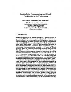
Figure 2 shows the basic framework of the PartMiner approach. It consists of two phases. At the first phase, a graph partitioning algorithm is used to split every graph in the dataset into smaller subgraphs. Then the subgraphs are grouped into units. The second phase applies an existing memory-based graph mining algorithm (used Gaston algorithm) to discover the frequent subgraphs in each unit. The set of frequent subgraphs in each unit are then merged via a merge-join operation to recover the complete set of frequent subgraphs.
G1
G2
G3
….
….
Proof: By an induction method.
Gn
“Base Case: n = 2. This is trivially true as shown in PartMiner paper. G11
G12 … G1k
G11 G21 … Gn1
U1
G21 G22 … G2k
G12
……
G22 … Gn2
…
P(U2)
…
U2 P(U1)
Gn1 Gn2 … Gnk
G1k
Uk
G2k …. Gnk
P(Uk)
P(D)
Induction Step: Suppose Hn is true, the authors want to show that Hn+1 is also true. If Hn is true, it is able to recover all subgraphs of a graph G of size n. Now one have a graph G’ of size n + 1. Graph G’ is partitioned into two subgraphs. Let G1 denote the partition of size n, and let G2 denote the partition of size i - 2, 3 < i < n (see Figure 3). All subgraphs from G1 (because G1 is of size n) can be recovered. Hence, the only missing subgraphs are those involving the edge (v1; v2) in G2. These subgraphs are formed by the joining of the subgraphs of G1 and G2, which share one of the common edges (v2; v3); …; (v2; vi) marked as grey in Figure 3. This step in fact is included in the merge-join operation. In other words, if Hn is true, then Hn+1 must be true”.
Figure 2: PartMiner partitioning framework j
G1
G’
3
Dividing Graph Dataset into Units PartMiner has adopted an approach that repeatedly bi-partitions each of the graphs in the dataset. For example, a graph G is first divided into 2 subgraphs G1 and G2, then G1 (G2) is again further divided into 2 subgraphs G11 and G12 (G21 and G22). This bi-partitioning process yields a total of 4 subgraphs for G. By applying this bi-partitioning procedure on each of the graphs Gi in the dataset, we can have four subgraphs Gi1, Gi2, Gi3, and Gi4 for each Gi. Each of the subgraphs Gij , 1 ≤ i ≤ 4, can be grouped into one unit Uj.
j
n
Combining Frequent Subgraphs At this point, the set of frequent subgraphs in the units have been computed. In PartMiner, a merge-join operation is defined to recover the complete set of frequent subgraphs in original graph dataset. The idea behind the merge-join operation is illustrated detail in PartMiner paper. Completeness of PartMiner approach Completeness means all frequent subgraphs in the dataset will be discovered independent from the partitioning technique. The completeness of PartMiner approach is claimed by three theorems as follows: Theorem 1: The set of subgraphs of a graph G (i.e. PS(G)) with size of n, n ≥ 2, can be fully recovered by recursively applying the merge-join operation on its bi-partitioned subgraphs G1 and G2.
2
n-1
1
2
i
n-1
i
G2
3
Vertices of shared edges
Figure 3: Induction step.
Mining Frequent Subgraphs in Units PartMiner approach uses the Gaston algorithm to find the set of frequent graphs in the units. After all P(Ui), 1 ≤ i ≤ k, are discovered, the combining step is applied to get full frequent subgraphs in the original dataset.
n
3
2
1
i
Theorem 2: (Apriori property) If a graph G is frequent in graph dataset D, all of its subgraphs are frequent in D. Proof: It is obviously according to subgraph definition. Thoerem 3: Let D be a graph dataset that has been divided into k smaller units Ui, k ≥ 2, 1 ≤ i ≤ k. If the complete set of frequent subgraphs P(Ui) in each unit Ui, 1 ≤ i ≤ k is already known, the complete set of frequent subgraphs P(D) in D can be determined. Proof: Also by induction method. This theorem is a key point to prove the completeness of PartMiner. However, we found that there is not a correct proof. We will come back with this statement in our following section.
5.2
Critical observations
After above review on PartMiner approach, we now show that in general, PartMiner provides incorrect mining results. Particularly, we shall prove that the Proof of Theorem 1 in PartMiner is incorrect and the proof of Theorem 3 in PartMiner is incorrect either.
Claim 5.1 (Incorrectness of Proof for Theorem 1) We think that the induction method is not suitable to prove Theorem 1. In the induction step, under the assumption that Theorem 1 is true for graphs with size n (Hn), the authors try to show that Theorem 1 is also true for graphs with size n+1 (Hn+1). An example is used for this purpose, as shown in Figure 3. However, this example is just a special case and is thus not general enough to be representative of all possible situations. The reasons are: It is assumed that the difference between G’ (i.e., size n + 1) and G (i.e., size n) is that there is a new vertex v1 in G’ because the authors claim that “the only missing subgraphs are those involving the edge (v1, v2) in G2”. After all, in Figure 3, v1 is only connected to v2. However, the size of a graph is determined by the number of edges instead of the number of vertices. In other words, G’ could also be constructed by adding a new edge between two existing vertices in G that are not originally connected. Note that this case can not be explained by Figure 3. Furthermore, in Figure 3, G’ is carefully partitioned so that G1 is of size n and G2 is of size i-2 with 3 < i < n. Compared to the definition of Theorem 1, this is also a special case of partition. In fact, the authors of PartMinner should show that Hn+1 is true for any two G1 and G2 resulted from any bipartition of G’. Counter example 1: Finally, an example is shown below (Figure 4) where G’ is of size n + 1 = 3. It is not sure whether Theorem 1 is true on G’ given the base case of induction method with n = 2. Note that G1 is of size n + 1 = 3 and G2 is of size n = 2. In the paper, the authors claim that G1 is of size n and G2 is of size i - 2 with 3 < i < n, which is impossible in this case, no matter how G’ is bi-partitioned.
3 3
2
G’
2
1
G1
1
3
1
2
G2
Figure 4: Counter example 1 of induction proof for Theorem 1
Correct proof: We prove by contradiction. Given a graph G partitioned by the method proposed in PartMiner approach into two subgraphs G1 and G2. Suppose the complete set of subgraphs of G1, PS(G1) and the complete set of subgraphs of G2, PS(G2), are given. We can recover the complete set of subgraphs of G by applying the merge-join operation in PartMiner.
Assume that there is a subgraph of G, denoted gs, but cannot recover from PS(G1) and PS(G2). Therefore, there is at least one 1-edge subgraph of gs, but cannot recover from the set of 1-edge subgraphs of PS(G1) and the set of 1-edge subgraphs of PS(G2). It is impossible because according to PartMiner’s bi-partitioning techniques, the set of 1-edge subgraphs of PS(G1) and the set of 1-edge subgraphs of PS(G2) contains complete set 1-edge subgraphs of original graph G. As a result, the proof of Theorem 1 is done. Claim 5.2 (Incorrectness of Proof forTheorem 3) We see there is no relationship between Theorem 1 and Theorem 3. Because, Theorem 1 is about the subgraphs of only one graph G, meanwhile Theorem 3 is about the frequent subgraphs of unit which is a set of graphs. Moreover, the set of frequent subgraphs in original dataset D is totally deferent from the set of subgraphs in each graph of D. We cannot generalize from only one graph (Theorem 1) to a set of graphs (Theorem 3). Therefore, the base case of induction step (k = 2) in the proof of Theorem 3 is incorrect. As a result, the induction step for k > 2 is failed as well.
Correct proof Assume that the min_sup threshold is a number of graphs (not percentage threshold). A graph dataset has been divided into k smaller units Ui, k ≥ 2, 1 ≤ i ≤ k. If the complete set of frequent subgraphs P(Ui) with min_sup / k threshold (according to PartMiner algorithm) in each unit Ui, 1 ≤ i ≤ k is already known, the complete set of frequent subgraphs P(D) in D can be determined by the merge-join operation. We prove by contradiction. Assume that there is a frequent subgraph of P(D), denoted fgs, but cannot determine from P(Ui), k ≥ 2, 1 ≤ i ≤ k. Therefore, there is at least one 1-edge subgraph of fgs which is frequent in D, denoted as f1gs, but cannot determine from the set of 1-edge subgraphs of P(U1), P(U2), … and P(Uk). As a result: supportD(f1gs) dataset D)
≥ min_sup (for the whole original
In every unit Ui, 1 supportUi(f1gs)