A Framework for Cross-layer Optimization of Video ... - CiteSeerX

A Framework for Cross-layer Optimization of Video Streaming in Wireless Networks CHENG-HSIN HSU and MOHAMED HEFEEDA School of Computing Science, Simon Fraser University, Canada

We present a general framework for optimizing the quality of video streaming in wireless networks that are composed of multiple wireless stations. The framework is general because: (i) it can be applied to different wireless networks, such as IEEE 802.11e WLAN and IEEE 802.16 WiMAX, (ii) it can employ different objective functions for the optimization, and (iii) it can adopt various models for the wireless channel, the link layer, and the distortion of the video streams in the application layer. The optimization framework controls parameters in different layers to optimally allocate the wireless network resources among all stations. More specifically, we address this video optimization problem in two steps. First, we formulate an abstract optimization problem for video streaming in wireless networks in general. This formulation exposes the important interaction between parameters belonging to different layers in the network stack. Then, we instantiate and solve the general problem for the recent IEEE 802.11e WLANs, which support prioritized traffic classes. We show how the calculated optimal solutions can efficiently be implemented in the distributed mode of the IEEE 802.11e standard. We evaluate our proposed solution using extensive simulations in the OPNET simulator, which captures most features of realistic wireless networks. In addition, to show the practicality of our solution, we have implemented it in the driver of an off-the-shelf wireless adapter that complies with the IEEE 802.11e standard. Our experimental and simulation results show that significant quality improvement in video streams can be achieved using our solution, without incurring any significant communication or computational overhead. We also explain how the general video optimization problem can be applied to other wireless networks, in particular, to the IEEE 802.16 WiMAX networks, which are becoming very popular. Categories and Subject Descriptors: C.2.1 [Computer-Communication Networks]: Network Architecture and Design General Terms: Design Additional Key Words and Phrases: Wireless networks, video optimization, cross layer design, effective airtime, WLAN, WiMAX

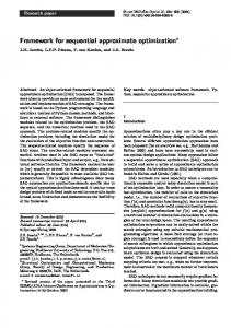
1. INTRODUCTION Wireless networks offer convenience, mobility, and low-cost infrastructure. As wireless networks provide higher throughput and quality-of-service (QoS), video streaming over wireless networks has become an important application. The optimization of video streaming over wireless networks, however, is a challenging task because of the heterogeneity and dynamic nature of the channels among wireless nodes [Katsaggelos et al. 2005]. In this paper, we seek to optimize the quality of video streaming in wireless networks with energy-constrained devices. We consider a general wireless network model, which is depicted in Fig. 1. In this model, there are multiple wireless stations sharing a common wireless medium. These wireless stations can, for example, be notebook computers, PDAs, or video sensors. The wireless medium can be cellular networks, IEEE 802.16 WiMAX networks, or IEEE 802.11e WLANs. The wireless stations can be sending and/or receiving video streams to/from the video server through a wireless base station. ACM Transactions on Multimedia Computing, Communications and Applications, Vol. V, No. N, September 2009, Pages 1–0??.

2

·

C. Hsu and M.Hefeeda Wireless Station

Wireless Station Base Station

High−Speed Link

Wireless Medium (WiFi, WiMAX, Cellular) Camera

Streaming Server or Video Procecssing Server

Wireless Station

PDA

Wireless Station

Laptop

Fig. 1.

A general model for video optimization in wireless networks.

For example, in video surveillance systems, video sensors capture and transmit their streams over a WLAN to a processing server for further analysis. As another example, wireless stations can be receiving video tutorials, demos, or movies from a video-on-demand streaming server over a WiMAX network. The model assumes that the video streaming or processing server is connected to the wireless base station through a high-speed link, e.g., Fast or Giga bit Ethernet link. Therefore, the server–base station link is not the bottleneck in the system. This is a typical setting for local and wide area setups for video streaming. For example, in streaming over a cellular network, the server–base station bandwidth is usually several order of magnitudes higher than the wireless channel bandwidth. In WLANs, the server can be attached to the base station through wired high-speed Ethernet switches, while all wireless stations compete with each other for the wireless channel, which has higher bit error rates and smaller bandwidth. Moreover, we consider batterypowered wireless stations that have power constraints. To cope with the power constraints, stations employ complexity scalable video coders that may selectively skip some encoding optimization modules to save power. To optimize quality at a given power budget, we employ models that relate power consumption, encoding bit rate, and resulting distortion. Power considerations are critical in wireless devices. Previous measurement studies indicate that modern video coders consume about two-thirds of the system power in video wireless communication systems [He et al. 2005]. We approach the video optimization problem in wireless networks in two steps. First, we formulate an abstract video optimization problem for general wireless networks composed of multiple stations. Second, we instantiate and solve the general problem for IEEE 802.11e networks. We present key models for different layers, and we formulate and solve the video optimization problem in the IEEE 802.11e networks. We then show how to enforce the calculated optimal allocation in the IEEE 802.11e networks, which leads to an efficient, distributed video optimization algorithm. We extensively evaluate the proposed algorithm using both simulations and real experiments, to cover various setups and system parameters, and show the practicality of the algorithm. The specific contributions in this paper can be summarized as follows: ACM Transactions on Multimedia Computing, Communications and Applications, Vol. V, No. N, September 2009.

A Framework for Cross-layer Optimization of Video Streaming in Wireless Networks

·

3

—We propose a general model for formulating video optimization problems to allocate the wireless resources in wireless networks. This model exposes the important interaction between parameters belonging to different layers in the network stack, and is fairly general. For example, various optimization criteria, such as minimizing average distortion and minimizing maximum distortion among wireless stations can be adopted. —We use the general model to instantiate an optimization problem for IEEE 802.11e networks, which support differential QoS. We chose IEEE 802.11e networks because they are distributed, and thus much more challenging than the centrally-controlled networks such as cellular and the IEEE 802.16 WiMAX networks. —We present key models for different layers in the IEEE 802.11e standard. More importantly, we develop a simple, closed-form, analytic model to estimate airtime allocation achieved by different MAC parameters. While this airtime model provides us an efficient way to differentially allocate network resources among wireless stations, it could be of interest in its own right for other applications in the IEEE 802.11e networks. —We solve the optimization problem for the IEEE 802.11e networks, and we propose a distributed algorithm, which is based on analytically derived closed-form formulas. This algorithm is in contrast to computationally intensive numerical methods used in previous works. In addition, we show how the calculated optimal allocations can be enforced using the airtime model in the distributed mode of the IEEE 802.11e standard. —We implement the distributed algorithm in the OPNET simulator, which captures most features of realistic wireless networks. We then use the OPNET simulator to extensively evaluate the algorithm under various channel conditions and video characteristics. —We implement the proposed distributed algorithm in the Linux driver of an offthe-shelf wireless adapter that is compliant with the IEEE 802.11e standard, i.e., supports quality differentiation. We then setup a real WLAN testbed, and use it to show the practicality and efficiency of the algorithm. —We also explain how our general model of the video optimization problem can be applied to other wireless networks, in particular, to the IEEE 802.16 WiMAX networks. Remark: Our modeling and solution of the video optimization problem are applicable only to wireless networks that do support some QoS differentiation among competing traffic streams. We build our cross-layer solution on top of the basic QoS differentiation scheme provided by such networks. In WiMAX networks [Cicconetti et al. 2006; Ghosh et al. 2005], for example, the base station can allocate different portions of the wireless channel to different stations. Also, as detailed in Sec. 4, the recent IEEE 802.11e standard [IEEE Std 802.11 2005] supports prioritized traffic classes. We should mention that our work is not applicable to the common IEEE 802.11 a/b/g networks, because they don’t support link-level traffic differentiation. Also, our work is not targeted towards the general Internet streaming systems in which some receivers are attached to the Internet via a WLAN. ACM Transactions on Multimedia Computing, Communications and Applications, Vol. V, No. N, September 2009.

4

·

C. Hsu and M.Hefeeda

Table I. Notations used in this paper. Notation Definition Notation Definition S number of wireless stations. µs picture complexity. B(·) D(·) ps rs V bs φs EA CW min CW max CW σs

air medium capacity. P-R-D function.

1/γ

g(ps ) = ps αs = σs2

1/γ

power level. βs = µs ys ps application layer rate. xs video characteristics. ls link layer bandwidth. os airtime fraction. tl effective airtime. tb minimum contention window. ts maximum contention window. td contention window size. ta standard deviation of raw picture.

power consumption. P-R-D parameter. P-R-D parameter. TXOP limit. average payload length. average overhead length. slot time. beacon interval. short inter-frame space. distributed inter-frame space. average time to send ACK.

Preliminary version of this paper appears in [Hsu and Hefeeda 2009]. The current paper contains significant additional materials and experiments, including a closedform analytic model to estimate airtime allocation in IEEE 802.11e networks, more comprehensive simulation designs and results, and generalization of the proposed model to consider different objective functions, among other improvements. The rest of this paper is organized as follows. In Sec. 2, we present the general model for video optimization in wireless networks. We then instantiate the video optimization problem for the IEEE 802.11e networks by first presenting the key models for various network layers in Sec. 3. We formulate and solve the video optimization problem in Sec. 4. In Sec. 5, we evaluate the proposed distributed algorithm using extensive simulations and experiments. We summarize the related works in the literature in Sec. 6. Last, Sec. 7 concludes the paper. 2. GENERAL SYSTEM MODEL In this section, we introduce a general system model for video streaming in singlehop wireless networks, where we demonstrate the interaction among parameters in different layers. Then, we formulate a cross-layer video optimization problem under this general model. Table I summarizes the notations used in this paper. As shown in Fig. 1, the model has S ≥ 1 wireless stations sharing a common wireless medium. The wireless stations are battery-powered. For concreteness, we focus on the case where the wireless stations transmit video streams to a video processing server that is co-located with the wireless base station, as in video surveillance systems. Similar analysis can be done when the base station transmits video streams to wireless stations. Each station encodes its video stream and competes with other stations for the wireless medium to send the video data to the server. The wireless stations are, in general, heterogeneous in their energy level and they are transmitting different streams. Furthermore, they could be at different distances from the base station and/or experiencing different noise and interference levels. Therefore, the channel rates between individual wireless stations and the base station are also heterogeneous. The goal is to optimize the overall video quality of all streams received by the server by properly allocating the wireless medium resources while not ACM Transactions on Multimedia Computing, Communications and Applications, Vol. V, No. N, September 2009.

A Framework for Cross-layer Optimization of Video Streaming in Wireless Networks Base Station

P−R−D Characteristics

Optimal Encoding Rate

·

5

Wireless Station

Complexity Scalable Video (De)coder

APP

QoS−Enabled Controller

LINK

Radio Module

PHY

Our Optimization

MAC Parameters

Algorithm

Optimal Airtime Allocation Optimal Share of Wireless Bandwidth Channel Rate

Fig. 2. The interaction among different layers to optimize video quality. Solid arrows indicate inputs to our algorithm, while dotted arrows show the outputs. Notice that the inputs and outputs belong to different layers.

exceeding the energy constraint of each station. We adopt a cross-layer approach to achieve this goal, as summarized in Fig. 2. In particular, our optimization scheme uses and sets parameters in three layers: application, link, and physical. In the application layer, complexity scalable video coding techniques, e.g., [He et al. 2005; Lu et al. 2003], are employed. These coding techniques are abstracted by the so-called Power-Rate-Distortion (P-R-D) models [Cheng et al. 2006; He et al. 2005]. A P-R-D model relates the expected distortion in the reconstructed video with the encoding rate and the power allocated to the encoding process. More power allocated to the encoding process allows it to use more sophisticated video encoding and compression algorithms, and thus results in better quality (i.e., lower distortion) at the same bit rate. Also, higher bit rates usually produce higher video quality, according to the shape of the P-R-D curve. Therefore, in our problem, a wireless station s (1 ≤ s ≤ S) employs a P-R-D model in the application layer to estimate the distortion D(ps , rs , V ) as a function of the allocated power level ps , the coding rate rs , and the video characteristics V . Our optimization method takes the function D(·), ps , and V as inputs, then computes the optimal encoding rate rs . We emphasize that D(·), ps , and V are not determined by our algorithm. For example, mobile devices often have a dedicate battery level monitor, which can determine the proper ps based on current battery level and other factors like per-bit energy consumption of the current modulation and channel coding scheme. The link and physical layers depend on the wireless medium technology. But in general, the physical layer can be modeled by the bit rate of the channel between the wireless station and the base station. The objective of the link layer is to coordinate the access to the shared wireless medium. That is, it needs to allocate the optimal share of bandwidth bs to each station s such that the aggregate bandwidth does not exceed the link capacity B. After computing the bandwidth share of each station, the system needs to enforce this allocation, i.e., allows each station to actually obtain its computed bandwidth. ACM Transactions on Multimedia Computing, Communications and Applications, Vol. V, No. N, September 2009.

6

·


The allocation enforcement scheme is much easier in centrally-controlled wireless systems, such as TDMA or FDMA cellular networks, than in distributed wireless systems, such as IEEE 802.11e WLANs. This is because in TDMA systems, for example, the base station can appropriately allocate time slots among wireless stations. Whereas, in a WLAN each station independently competes for bandwidth according to the distributed 802.11e MAC protocol. As shown in Fig. 2, the link layer parameters and the physical channel rate are given to our optimization method, the optimal share of bandwidth for each station is produced by the optimization method. Furthermore, our optimization method specifies how these bandwidth shares can be achieved by wireless stations. As will be detailed later, we present simple and distributed solution for this optimization problem in which the base station and wireless stations cooperate to compute the optimal solution without imposing any significant traffic overhead. Finally, the cross-layer video optimization problem considered in this paper can be stated as follows. Find the optimal policy Φ∗ = {φ∗s = (rs∗ , b∗s ) | 1 ≤ s ≤ S} such that: P G : Φ∗ = arg min Φ

s.t.

S X

D(ps , rs , V )

(1a)

S X

bs ≤ B(·);

(1b)

s=1

s=1

s = 1, 2, . . . , S.

(1c)

The objective of this formulation is to minimize the overall distortion for all wireless stations. The wireless medium capacity B(·) is a function of the number of wireless stations, the protocol used in the link layer, and the channel physical rates between wireless stations and the base station. Since B(·) captures the physical and link layer parameters and D(·) captures the application parameters, solving the general problem P G in Eq. (1) will yield a cross-layer optimized solution for video streaming in wireless networks. Problem P G is fairly general, and various models for D(·) and B(·) can be plugged into it. The solution may be obtained analytically for some cases and can be computed numerically for others. We show in the rest of this paper how we instantiate P G for the IEEE 802.11e WLANs and how we solve it. As discussed above, solving the problem for the IEEE 802.11e standard is challenging due to the distributed nature of the protocol, which makes estimating the wireless medium capacity B(·) and enforcing the computed optimal bandwidth allocations more difficult. Solving the problem for centrally-controlled networks such as TDMA and WiMAX can be done in a similar, but much easier, way, as outlined in Sec. 7. We also mention that P G is applicable in solving the video optimization problem when the base station is transmitting to multiple stations. In this case, ps represents the power spent by station s to receive and decode its video stream. Therefore, this abstract formulation of the video optimization problem in wireless networks could be useful in different settings. We should mention that to transmit multiple nonscalable video streams to different wireless stations at different bit rates, the base station must transcode each ACM Transactions on Multimedia Computing, Communications and Applications, Vol. V, No. N, September 2009.


·

7

video stream to its target bit rate, which is computationally intensive. In contrast, adopting scalable coded streams allows the base station to efficiently scale each stream to its target bit rate [Schwarz et al. 2007]. Since the stream scaling is efficient, a base station can provide real-time rate adaption for a large number of wireless stations. Sending scalable coded streams also enables wireless stations to selectively decode partial streams to save energy. More precisely, a recent paper proposes a complexity model for decoding scalable streams [Ma and Wang 2008], which enables video decoders to opt for partial streams for lower computational complexity, thus lower energy consumption. Different Objectives: Problem P G employs an objective function Eq. (1a) that minimizes the average reconstructed video distortion among all mobile stations. This objective function, also known as MMSE (minimum average distortion), is the most widely used objective function in many video optimization problems [Ortega and Ramchandran 1998]. However, other objective functions, such as MMAX (minmax distortion) that minimizes the maximum distortion among all mobile stations, may be more appropriate in other applications. Problem P G can adapt to these applications by replacing Eq. (1a) with the new objective function, e.g., in the MMAX case, the following objective function should be used: S

Φ∗ = arg min max D(ps , rs , V ). Φ

s=1

With a proper objective function, the general system model and Problem P G can be used in those applications as well, while the resulting formulation can be solved using similar techniques presented in this paper. 3. MODELS FOR 802.11E WLANS The IEEE 802.11 wireless LAN standard is widely deployed in many real systems. Although the legacy IEEE 802.11 a/b/g standards [IEEE Std 802.11 1999] do not support link layer QoS, the recently-finalized IEEE 802.11e standard [IEEE Std 802.11 2005] enables QoS differentiation among different applications [Kim et al. 2007; Gao et al. 2005; Ni 2005]. The IEEE 802.11e standard defines two medium access modes: contention-based and polling-based contention-free. In the contentionfree mode, a station sends its QoS requirements (e.g., mean rate, peak rate, and maximum burst size) to the base station, which decides whether to admit or reject the station’s request based on the available resources. The contention-free mode requires centralized admission and scheduling algorithms, thus is not flexible [Chou et al. 2005]. In addition, it may not fully utilize the channel bandwidth, because it relies on resource reservations, which are typically made for worst case scenarios. In this work, we build our solution on top of the more flexible contention-based access mode, which is known as the Enhancement Distributed Channel Access (EDCA) mode. Our work can easily be extended to support the contention-free mode as well. In this case, the base station solves the optimization problem and centrally allocates the bandwidth to wireless stations. Fig. 3 lists the parameters used in the video optimization problem in IEEE 802.11e WLANs. We discuss each of these parameters in details in the following subsections. We start by introducing the physical layer model employed in this paper. Then, we present the main QoS features of the EDCA mode of the IEEE ACM Transactions on Multimedia Computing, Communications and Applications, Vol. V, No. N, September 2009.

8

·


Application Layer (streaming) rs : Encoding rate (o/p) ps : Normalized power level Ds : Video distortion

Link Layer (802.11) CW : Contention window AIFS : Arbitration inter-frame space TXOP: Transmission opportunity limit (o/p)

Physical Layer Modulation scheme ys : Physical layer rate Fig. 3.

The parameters used in optimizing video quality in IEEE 802.11e WLANs.

802.11e link layer standard, where we describe the controlling parameters used in our optimization problem. Finally, we propose a simple model for estimating the wireless link capacity, which we will use in our optimization problem.

3.1 Physical Layer Model Most modern WLAN adaptors support multiple physical modes to cope with different channel conditions, such as various signal fading and interference levels. Each physical mode specifies a modulation scheme and a channel coding algorithm. A channel adaptation algorithm determines the optimal physical mode that maximizes the effective throughput. This channel adaptation algorithm is usually based on signal strength measurements and bit error rates, and does not depend on information from upper layers. Thus, our video optimization problem does not try to control the physical layer rate, in order to avoid interfering with the channel adaptation algorithm typically implemented in the firmware. We use ys to denote the physical rate at station s (1 ≤ s ≤ S), which is decided by the channel adaptation algorithm. ys is not assumed to be static, rather, it varies based on channel conditions and characteristics of station s itself, such as its mobility pattern and its distance from the base station. We do not control ys in our optimization problem. We denote the application layer rate of station s by rs . To analyze the interaction between rs and ys , let us ignore overheads such as protocol headers and acknowledgment frames. We will relax this assumption later. Define φs = rs /ys . Since there is at most one successful transmission at any moment without colliding with other transmissions, φs can be seen as the fraction of airtime assigned to station s. For illustration: to stream a 1-Mbps coded stream over a 10-Mbps channel, the station has to acquire at least 10% of the airtime. Clearly, the total effective airtime (EA), i.e., the airtime during which useful data is transmitted and no collision occurs, is limited. The value of EA depends on the details of the link layer protocol and the number of stations, as described in the following subsections. ACM Transactions on Multimedia Computing, Communications and Applications, Vol. V, No. N, September 2009.


·

9

3.2 Link Layer Model In EDCA mode, packets are categorized into prioritized classes, called access categories (ACs). For example, audio, video, and best effort traffic could make three different ACs. Traffic sessions compete with each other for the wireless medium. In EDCA mode, airtime allocation among traffic session in different ACs is differentiated by assigning each AC different EDCA parameters. Differential allocation of airtime to different ACs is essential for QoS-enabled applications. For example, some traffic sessions belonging to the video AC may need to be allocated larger fractions of the airtime than traffic sessions belonging to the best-effort AC. There are two sets of EDCA parameters that can achieve airtime differentiation. The first set controls the frequency of acquiring a transmission opportunity on the wireless medium, while the second set controls the duration of an acquired transmission opportunity. The frequency of transmission opportunities is determined through three parameters: arbitration inter-frame space (AIFS ), minimum contention window size (CW min ), and maximum contention window size (CW max ). Each AC maintains a contention window size variable (CW ), which is initialized to CW min . The CW is incremented after transmission failures until it reaches CW max , and is reset to CW min after a successful transmission. To avoid collisions, a backoff timer is independently chosen from the range [0, CW ] for each AC. Since smaller CW min and CW max generally lead to smaller CW values, they result in shorter backoff timer and higher transmission opportunity frequency. Moreover, the backoff timer is decremented once the wireless medium is sensed idle for at least AIFS seconds. Smaller AIFS values enable wireless stations to start decrementing backoff timers earlier, and thus increase the transmission opportunity frequency. On the other hand, the maximum allowed duration for each acquired transmission opportunity is determined by a parameter called the TXOP limit. Once a station acquires a transmission opportunity, it may transmit multiple frames within the assigned TXOP limit. Assigning different TXOP values to ACs, therefore, achieves differential airtime allocations. The above mentioned EDCA mode supports per-class (AC) differentiated service, but it does not support per-session QoS, which is important to video communications. For example, some video sessions may need to be allocated larger fractions of the airtime than others in the same AC, because the wireless stations transmitting them are farther away from the base station or they have poorer channel conditions. To cope with this limitation of IEEE 802.11e EDCA mode, we propose to control the EDCA parameters of different traffic sessions in the same AC such that the differential airtime allocation among traffic sessions is achieved. More precisely, to achieve a given airtime allocation φs , we can either fix the frequency-related parameters among stations and use the transmission opportunity limit as the control knob, or fix the transmission opportunity limit among stations and use the frequency-related parameters as the control knob. The experiments in [Chou et al. 2005] indicate that both approaches result in similar airtime differentiation behavior. However, the frequency-based approaches incur high computational complexity because modeling the AIFS , CW min and CW max values and their impacts on throughput is complicated. There are several models in the literature ACM Transactions on Multimedia Computing, Communications and Applications, Vol. V, No. N, September 2009.

10

·


for throughput estimations. All these models require solving nonlinear equation systems that are extremely computationally demanding and not suitable for realtime applications, see for example [Hui and Devetsikiotis 2005] and the references cited therein. In our video optimization problem, we control the TXOP limit of wireless stations, and we fix all frequency-related parameters (AIFS , CW min , and CW max ). As shown in the next subsection, controlling the TXOP limit allows us to derive a simple, closed-form equation for the effective airtime, which makes our optimization problem less complex without sacrificing the optimal solution. In the evaluation section, we use a real 802.11 testbed to verify that controlling the TXOP limit is practically easier and it indeed achieves the desired differential allocation of the wireless medium. 3.3 Effective Airtime Model In the previous subsection, we discussed how the TXOP limit parameter of the IEEE 802.11e standard can be used to differentially allocate airtime among wireless stations. In our video optimization problem, we need to determine the total effective airtime (EA) of the wireless medium so that we can divide it among stations, and to avoid over/under allocation of the wireless medium. We develop a simple, closed-form, analytic model to estimate EA. The model accounts for the number of wireless stations in the system as well as the detailed operation of the EDCA mode, including collisions, backoffs, and the minimum and maximum sizes of the contention window. Our analysis is based on the analytic model proposed in [Ge et al. 2007], which has been verified by its authors using extensive simulations. The model in [Ge et al. 2007], however, does not work in the considered video streaming network for two reasons. First, their model assumes that the TXOP limit is fixed at small values and uniform across wireless stations. Our system, however, explicitly varies the TXOP limit to achieve per-stream airtime differentiation. The variability of the TXOP limit, as discussed below, is an important factor in determining accurate EA values. Second, their model analyzes the airtime for mixed traffic from multiple access categories, which renders it too complex to be run in real-time. Therefore, their algorithm in not suitable for video streaming networks. In contrast, we develop a new EA model in the following, which considers TXOP limit variability and can be efficiently calculated. Lemma 1 Effective Airtime Model. Consider S wireless stations compete for the shared air medium of a wireless LAN using the IEEE 802.11e EDCA protocol. These wireless stations transmit video data to/from the base station at different bit rates. The video traffic is the dominating traffic in this wireless LAN, and the rate differentiation is achieved by varying the TXOP limits for individual wireless stations. The effective airtime can be approximated by: 1 , where CW min is the minimum conEA = 2 2S )S−1 )(1 − 1+( CW min + 2 CW min tention window size. Proof. We consider a p-persistent version of the EDCA protocol, which employs a backoff timer selection scheme different from the standard EDCA [Ge et al. 2007]. ACM Transactions on Multimedia Computing, Communications and Applications, Vol. V, No. N, September 2009.


·

11

While the standard EDCA uniformly selects backoff timers from an exponentially growing contention window, the p-persistent EDCA draws its backoff timers from a geometric distribution with parameter p. The p-persistent EDCA is more tractable than the standard EDCA because of its stateless nature. In addition, it has been shown that the standard EDCA minimum contention window size CW min can be converted to the p-persistent EDCA contention parameter p using the equation: p = 2 CW min +2 . This enables us to use the p-persistent EDCA to develop the performance model, and then obtain the performance model of the standard EDCA using simple substitution. In the p-persistent EDCA, we define the virtual transmission time vj as the time duration between the j-th and the (j + 1)-th successful transmissions. Each virtual transmission consists of three periods: idle, collision, and transmission. The idle period happens when all wireless stations are waiting for their backoff timers to expire. The collision period happens when more than one station initiate transmissions. The idle and collision periods may appear more than once in a virtual transmission, while a single transmission period occurs during a virtual transmission. We use E[x] to denote the average transmission opportunity limit for all wireless stations, and E[v] to denote the average virtual transmission time. Then, the effective airtime can be given by: EA = E[x]/E[v]. That is, the effective airtime is given by the ratio of the actual (useful) transmission time to the total transmission time after including all contention overheads, which are modeled by the virtual transmission time. We next compute E[v], by averaging the durations of collision and idle periods during a virtual transmission time. First, let us denote the number of collisions in a virtual transmission time by C. We also define ik to be the duration of the k-th idle period, and similarly, ck to be the duration of the k-th collision period. Then E[v] is given by: E[v] =E

C X

k=1

(td + ik + ck + ts + ta ) + E[iC+1 ] + E[x] + td

= E[C](E[c] + td + ts + ta ) + (E[C] + 1)E[i] + E[x] + td ,

(2)

where td is the distributed inter-frame space (DIFS), ts is the short inter-frame space (SIFS), and ta is the average time of sending an acknowledgment. In the above equation [Chou et al. 2005]: (i) The first summation represents the total time occupied by the idle and collision time before the transmission period; (ii) The second term represents the idle time just before the transmission period; (iii) The third term represents the successful transmission opportunity; (iv) The last term represents the DIFS interval between two adjacent virtual transmissions. Following [Ge et al. 2007] and using our single EDCA access category assumption, E[C], E[i], and E[c] can be shown to be given by the following equations: (1 − p)S 1 − (1 − p)S − 1, E[i] = tl , S−1 Sp(1 − p) 1 − (1 − p)S S j S S−j X j p (1 − p) E[f ] E[c] = , 1 − (1 − p)S − Sp(1 − p)S−1 j=2 E[C] =

(3)

ACM Transactions on Multimedia Computing, Communications and Applications, Vol. V, No. N, September 2009.

12

·


0.2

ρ/E[x]

0.15

CW min = 15 CW min = 31 CW min = 63

0.1

0.05

0 0

2

4 6 8 Number of stations

10

12

Fig. 4. The average values of ρ/E[x] for different numbers of wireless stations and various sizes of the minimum contention window.

where E[f ] is the average frame transmission time. The above calculation of E[v] and its components does not consider the length variability of the TXOP limit. Specifically, it does not consider the situation when a wireless station freezes its backoff timer because another station is transmitting during its TXOP limit, which may not be a small constant in our system. We call this freeze period as blocking duration. Note that, this blocking is different from the collision time duration E[c] in the sense that a collision only lasts for a frame-time but blocking lasts for up to a complete transmission opportunity limit, which can be significantly longer than the frame time. We compute the average blocking duration as follows. The probability that only one station is transmitting is: Sp(1 − p)S−1 . Since the average length of transmission opportunity limit is E[x], the expected value of the blocking duration is thus: Sp(1 − p)S−1 E[x]. Adding this blocking duration to the E[v] in Eq. (2), and re-arranging the formula, we get: E[v] = ρ + E[x](1 + pS(1 − p)S−1), where ρ = E[C](E[c] + td + ts + ta ) + (E[C] + 1)E[i] + td. Substituting p = 2/(CW min +2) in E[v], we get the effective airtime of the standard EDCA system as: EA =

1 ρ 2S 2 )S−1 + 1+( )(1 − E[x] CW min + 2 CW min

(4)

The above equation for EA can further be simplified by choosing any CW min ≥ 3, which is quite practical considering the range of CW min is between 1 and 1024. Under this assumption, the first term in the denominator is much smaller than the second term, and therefore, can be ignored. For example, if CW min = 3, the ρ/E[x] values are 0.0046, 0.0105, 0.0200 for 2, 3, 4 wireless stations, respectively. Moreover, the second term in the denominator of Eq. (4) is always greater than 1. To further validate this simplification, we numerically compute the values of ρ/E[x] with typical wireless system parameters and with random TXOP limits. We vary the CW min values and number of stations, and repeat the experiments 1000 times. We then compute the average value ρ/E[x], and we plot the results in Fig. 4. The figure shows that the ρ/E[x] values are indeed very small. Furthermore, ACM Transactions on Multimedia Computing, Communications and Applications, Vol. V, No. N, September 2009.


·

13

the minimum contention window size can be chosen to make the expected value of ρ/E[x] arbitrary small for a given number of stations. This does not impact the operation of the EDCA protocol, because CW min is fixed in all wireless stations belonging to the same access category, and the airtime differentiation comes from controlling the TXOP limit. Hence, we ignore ρ/E[x] in Eq. (4), which yields this lemma. We use the model presented in this lemma to solve the video optimization problem, in which the video traffic is the dominating traffic in the wireless LAN. We mention that the considered video streaming system controls the EDCA parameters for all access categories, and it sets the parameters in a way that video traffic has the highest priority. Since other traffic types are not as bandwidth intensive as video streams, and are given lower priority, they would not interfere with the video traffic. Finally, if a certain amount of bandwidth should be reserved for background traffic, we can reduce the EA value computed by Lemma 1. This is because the computed EA value is the maximum airtime that can be achieved by the wireless LAN assuming the background traffic is insignificant. 4. VIDEO OPTIMIZATION IN 802.11E WLANS In this section, we instantiate and solve the general video optimization problem presented in Sec. 2 for the IEEE 802.11e WLAN. We start by presenting the problem formulation, followed by our solution. Then, we show how the computed optimal solutions can be enforced by setting the appropriate parameters in the wireless stations. Finally, we present a simple algorithm to coordinate the interaction between the wireless stations and the base station to implement the computed optimal airtime allocations. 4.1 Problem Formulation Using the notations developed in Sec. 3, our problem can be stated as follows. Find the optimal airtime allocation Φ∗ = {φ∗s = rs∗ /ys |1 ≤ s ≤ S} that achieves the minimum average distortion for all wireless stations. Mathematically, P : Φ∗ = arg min Φ

s.t.

S X

D(ps , rs , σs , µs )

(5a)

S X

φs ≤ EA;

(5b)

s=1

s=1

rs = φs ys ;

(5c)

0 ≤ φs ≤ 1; s = 1, 2, . . . , S.

(5d) (5e)

In the first constraint Eq. (5b), EA is given by Eq. (4). This constraint prevents us from over-allocating the airtime. The second constraint Eq. (5c) follows from our discussion in Sec. 3.1 on the relationship between the application layer rate rs , the physical channel rate ys and the airtime fraction allocated to each station s. Solving this optimization problem yields an allocation that specifies the optimal airtime fraction φ∗s for each station s, from which we can compute the application ACM Transactions on Multimedia Computing, Communications and Applications, Vol. V, No. N, September 2009.

14

·


layer rate rs∗ . Therefore, the solution of our optimization problem jointly determines the best airtime allocation in the link layer and the best video coding rate in the application layer. 4.2 Problem Solution To solve the optimization problem in Eq. (5), we need to specify the P-R-D model to compute D(·). Any P-R-D model can be used in this problem. We present below the solution for the recently proposed model in [Cheng et al. 2006], which has been shown to be accurate for different types of video sequences [He et al. 2005]. Solutions for other P-R-D models can be done in similar ways. We emphasize that our video optimization problem is not restricted to the P-R-D model in [Cheng et al. 2006]. However, developing new P-R-D models is outside the scope of this paper, and is considered as a future work. We consider that each station s allocates a power budget ps to its video coder to encode its raw sequence at rate rs . The P-R-D model gives the distortion estimation as [Cheng et al. 2006]: D(ps , rs , σs , µs ) = σs2 2−µs rs g(ps ) ,

(6)

where σs2 is the video sequence variance, µs represents the encoder efficiency, and the function g(ps ) models the mapping between the video coder complexity and 1/γ the microprocessor power consumption. This function is given by: g(ps ) = ps , where 1 ≤ γ ≤ 3 is a system parameter. Both σs and µs are sequence dependent variables. σs2 is the variance of raw pictures, which can be derived at different aggregation levels, such as frame, group of picture, scene, and sequence. µs indicates the hardness of compressing the subject sequence, which can be estimated based on the observation on the correlation between µs and the degree of motion activities. Details of efficiently estimating σs , µs and more discussion on their characteristics are given in [Cheng et al. 2006]. We first show that our optimization problem is a convex programming problem in the following lemma, which will enable us to develop an efficient solution for it. Lemma 2. The video optimization problem in Eq. (5) is a convex programming problem, whose local minimum is also a global minimum, when the P-R-D model in Eq. (6) is used. That is, this optimization problem has a unique optimal solution. Proof. We notice that all constraints are linear functions. The proof is, therefore, reduced to show that the objective function is a convex function. Recall that the P-R-D model is given as: D(ps , ys φs , σs , µs ) = σs2 2−µs rs g(ps ) . For ease of presentation, we rewrite it as: D(ps , ys φs , σs , µs ) = αs 2−βs φs , where αs = σs2 , and 1/γ βs = µs ys ps . We observe that αs is always positive. This is because natural video sequences do not have zero-input variance. In addition, a zero input variance synthetic sequence is simple to compress at virtually zero power consumption, and therefore it is not of interest to the optimization problem. Furthermore, βs is also positive. This is because the compression hardness parameter µ is positive as shown by the estimation method given in [Cheng et al. 2006]. Meanwhile, zero ys or ps indicate that the wireless station s has no transmission or processing power. Thus, nothing can be done to improve its video quality. We, therefore, can exclude that station ACM Transactions on Multimedia Computing, Communications and Applications, Vol. V, No. N, September 2009.


·

15

from the optimization problem without negatively affecting the optimality of the resulted optimal airtime allocations. Given that αs , βs > 0, we know that the distortion αs 2−βs φs is a convex function with respect to φs . Hence, the objective function Eq. (5a), which is a non-negative weighted sum of convex functions, is also a convex function. This lemma enables us to solve our optimization problem as a convex programming problem. We present our solution in the next lemma. Lemma 3. The optimal airtime allocation Φ∗ for the video quality optimization problem in Eq. (5) is given by: φ∗s = −

S S X X 1 log2 αs βs ln 2 ˆ=( − EA)/( ). where log2 λ β β s s=1 s s=1 (7)

ˆ λ 1 log2 , βs αs βs ln 2

Proof. This is a budget-constrained convex programming problem, which can be solved using Lagrangian relaxation techniques [Ortega and Ramchandran 1998]. We write the following Lagrangian-relaxed formulation: P LB : Φ∗ = arg min Φ

S X s=1

S X D(ps , φs ys , σs , µs ) + λ( φs − EA) , s=1

where 0 ≤φs ≤ 1; s = 1, 2, . . . , S.

(8)

for a nonnegative Lagrangian multiplier λ. Observe that for a given λ value, every wireless station s can compute its optimal airtime fraction, denoted as φ∗s , in a distributed manner. Mathematically, φ∗s at station s is given by solving this subproblem: P S : φ∗s = arg min D(ps , φs ys , σs , µs ) + λφs , where 0 ≤ φs ≤ 1, φs

(9)

where the only information shared among wireless stations is the λ value. Thus, solving this problem requires a very small communication cost and is efficient. The optimal solution, φ∗s , can be derived by: ∂(αs 2−βs φs + λφs )/∂φs = 0, which yields φ∗s = −

1 λ log2 . βs αs βs ln 2

(10)

This formula gives us the unique extreme point φ∗s for station s. It is straightforward to see that the second derivative of the objective function of problem P S is larger than zero. Thus, φ∗s is indeed the airtime fraction that minimizes the distortion of the video sequence sent by station s. Since the total distortion is computed by the linear summation operator, minimizing distortion at each station will yield the minimal total distortion. We next search for the optimal P λ value. In the Lagrangian-relaxed problem S Eq. (8), tightening the constraint s=1 φs ≤ EA results in an optimal solution for the original problem Eq. (5) as long as the solution is feasible in the original problem. This is intuitive because higher airtime fractions lead to lower distortion. ACM Transactions on Multimedia Computing, Communications and Applications, Vol. V, No. N, September 2009.

16

·


ˆ to denote this optimal λ value. We then derive λ ˆ as follows: We use λ S X

φs = EA

S X

−

s=1

ˆ 1 λ log2 = EA βs αs βs ln 2 s=1 PS log2 αs βs ln 2 − EA s=1 βs ˆ . ⇒ log2 λ = PS 1

⇒

(11)

s=1 βs

Notice that the optimal value φ∗s for any station s can be computed locally by that ˆ Furthermore, the computation is very simple and requires no station if it knows λ. matrix operations. Therefore, optimal airtime allocation among all stations can be achieved efficiently and in a distributed manner using a simple algorithm (presented in Sec. 4.4). 4.3 Parameter Setting After solving the optimization problem, we need to set the parameters in the application and link layers to enforce the computed optimal allocations. In the application layer, the optimal encoding rate is set as rs∗ = φ∗s ys for each station s. In the link layer, we need to allocate the airtime. As mentioned in Sec. 3, we use the transmission opportunity limit TXOP as the control knob to assign airtime among wireless stations. TXOP limits are set every beacon interval, which is defined by the standard. We fix all other parameters, so that the wireless stations have equal probability to obtain a transmission opportunity. We define x∗s as the TXOP limit for station s. Following similar derivation in the literature, such as [Shankar N and van der Schaar 2007; Chou et al. 2005], we compute x∗s as a function of φ∗s and protocol overheads as follows. We use ls to denote the average payload length of video packets sent by station s. We define os to be the mean header overhead of packets from station s. The overhead os includes headers from all network layers, such as application, transport, and data link headers. The frame size is, therefore, ls + os on the wireless channel. Since s the physical rate of station s is given as ys , it takes lsy+o seconds to transmit a s frame. We define tb to be the beacon interval, tl to be the slot time, ts to be the short inter-frame space (SIFS), td to be the distributed inter-frame space (DIFS), and ta to be the average time of sending an acknowledgment. Since WLANs cover a short range, propagation delays are negligible. To achieve the target application rate rs∗ , the number of data frames need to be sent in each beacon interval is given r∗ t as: ⌈ sls b ⌉, where rs∗ tb represents the application data amount. Since φ∗s = rs∗ /ys , φ∗ y t

the number of data frames is given as: ⌈ s lss b ⌉. In each transmission opportunity, the sender sends a data frame and waits for an acknowledgment frame from the receiver. Upon receiving a data frame, the receiver waits for a SIFS period, then sends an acknowledgment frame. Once this frame arrives at the sender, the sender waits for a SIFS period and sends another data ACM Transactions on Multimedia Computing, Communications and Applications, Vol. V, No. N, September 2009.


·

17

frame given that its transmission opportunity limit is sufficient to accommodate that data frame and the expected acknowledgment frame. Otherwise, the current transmission opportunity ends. x∗s is therefore given by: ∗ ∗ ∗ φ y s tb φs ys tb ls + os φs ys tb + 2 s x∗s = − 1 ts + ta . (12) ls ys ls ls In the above equation, the first term accounts for the transmission time of data frames, the second term represents all SIFS periods, and the last term considers the transmission time of acknowledgment frames. 4.4 Optimal Allocation Algorithm In the previous subsections, we showed how the cross-layer optimization problem can be solved and how the parameters can be set in different layers. Now, we present an algorithm to implement the optimal solution by the wireless stations and the base station. The allocation algorithm is executed periodically. This period is set as multiple of the system beacon interval, because the EDCA parameters are announced using beacon frames. Clearly, the length of this period poses a trade-off: the more often the allocation algorithm is executed, the more responsive it is to channel and station conditions, but with higher computation and communication costs. Each wireless station s reports to the base station its αs and βs parameters, which depend on current power level, channel conditions, and sequence characteristics. The αs , βs values are reported initially and whenever they change. If there is no change in them, the station does not send anything, and the access point ˆ from Eq. (11), which is the uses previous values. The access point computes λ only information needed by wireless stations to compute their optimal allocations. Each station s uses Eq. (10) to computes φ∗s , from which it can set rs∗ as φ∗s ys , and compute x∗s from Eq. (12). There are two types of overheads imposed by our allocation algorithm: computation and communication. Since the solution is computed from closed-form equations, the computation cost is negligible compared to the video compression ˆ operations. The communication cost involves two parts. First, broadcasting the λ value to all stations. This single value can be included in the beacon frame (in the 64-bit information element field of the frame [Ge et al. 2007]) that is automatically sent by the access point every beacon period, or in the worst case, an additional packet is broadcast every beacon period. The second communication cost is transmitting αs , βs from each station to the access point. These values are sent by a station only whenever they change. In the worst case, there is a single packet for each station every beacon period. This is again a negligible cost compared to the video traffic. Therefore, our proposed method can optimize the video quality without incurring any significant overhead. 5. EVALUATION In this section, we first evaluate our allocation algorithm using the OPNET simulator under dynamic and realistic environments. Then, we show that our algorithm is practical by implementing it in off-the-shelf wireless adapters as a proof-of-concept. ACM Transactions on Multimedia Computing, Communications and Applications, Vol. V, No. N, September 2009.

18

·


5.1 OPNET Simulation Setup We evaluate our proposed allocation algorithm using the OPNET Modeler simulator version 12 [Modeler Web Page 2008]. The OPNET Modeler provides a simulation environment that accounts for the detailed operation of wireless networks, and is the most widely used commercial simulation environment. OPNET Modeler is written in C++, supports a comprehensive list of protocols, and allows users to develop customized, extended network nodes. We have implemented two new OPNET Modeler nodes: power-aware wireless station (WS) and intelligent base station (BS). We construct a wireless network with a BS and several WSes. Upon joining the network, each WS continuously streams a video sequence to the video server colocated with the BS. This video streaming traffic is tagged as video access category, as defined in the 802.11e standard. To simulate more realistic wireless environments, we have implemented the log-normal path loss model [Rappaport 1996, Chap 3.11] in OPNET. OPNET uses the much simpler free-space signal propagation model by default. We choose the path loss exponent to be 2.2 and the log-normal standard deviation to be 8.7 dB based on the recommendations in [Rappaport 1996, p.127]. Using this more elaborate path-loss model allows us to conduct simulations that are closer to real wireless systems. If not otherwise specified, we program each WS to join the network at the start of simulation and stay in the network until the simulation is finished. Upon joining the network, each WS sends a current status report to the BS. This status report consists of several parameters, such as P-R-D characteristics and the current modulation scheme of that WS. The BS, once receiving this report, invokes one of the considered airtime allocation algorithms and constructs a reply to that WS. This reply contains the assigned airtime allocation that instructs individual WSes to gauge their streaming rates and link-layer QoS parameters to achieve the highest average streaming quality for all WSes. In order to accommodate the dynamic environments, WSes periodically (every five seconds) send update reports to BS. We then collect statistics at the video server for individual WSes. Furthermore, we simulate scenarios where there is cross-traffic running through the WLAN and interfering with the video sessions. Next, we consider dynamic channel conditions due to node mobility. We also simulate another dynamic condition, in which several (up to 32) WSes sequentially joining the streaming network. Finally, we show the potential of energy saving using the considered P-R-D model. We have implemented four airtime allocation algorithms in OPNET. We first consider a scheme that equally divides available airtime among all WSes. This scheme is equivalent to using the IEEE 802.11e EDCA mode and assigning all video traffic a higher priority class than other traffic. That is, all video traffic session will belong to the same access category (AC), and will receive preferential access to the wireless channel than other types of traffic. However, since all video traffic sessions belong to the same AC and share the same EDCA parameters, they have similar chance to acquire the shared air medium. We refer to this algorithm as EDCA in the figures, because it represents what the IEEE 802.11e standard can achieve if it is used in a QoS-enabled WLAN. We have implemented our algorithm that is provably optimal as shown in Sec. 4.2. We denote our algorithm as OPT in the figures. We have also designed two other algorithms that improve upon EDCA, but ACM Transactions on Multimedia Computing, Communications and Applications, Vol. V, No. N, September 2009.


Fig. 5.

·

19

The simulated WLAN setup to evaluate the potential quality improvement.

not in a complete cross-layer manner, as our OPT algorithm does. These two algorithms are referred to as Ap-only and Link-only. The Ap-only algorithm allocates the wireless medium bandwidth among WSes in R-D optimized fashion, without considering the physical layer conditions. Whereas the Link-only algorithm only accounts for the link-layer status and it does not consider the R-D characteristics of the video streams. Comparisons with Ap-only and Link-only algorithms show the importance of considering information from multiple layers in optimizing the video quality in wireless networks. We should mention that we are not aware of any existing algorithms that solve our optimization problem, which considers real-time nonscalable video streaming from heterogeneous wireless stations to a base station over contention-based wireless networks (see Sec. 6 for details). Nevertheless, this is not an issue as our OPT algorithm is provably optimal. Moreover, we compare OPT algorithm against Ap-only and Link-only algorithms, which are not naively designed: They follow the traditional divide-and-conquer approach and search for optimal solutions within one layer of the network stack. 5.2 OPNET Simulation Results Potential Quality Improvement: We first compare our OPT algorithm against the EDCA algorithm. We deploy a BS and six WSes in a 300-meter by 300-meter area, as illustrated in Fig. 5. We consider heterogeneous channel conditions and P-RD characteristics. WSes that are closer to the BS have better channel conditions and thus can choose more aggressive modulation and coding schemes. Therefore, WSes closer to the BS have higher physical rates. Furthermore, each WS randomly chooses its P-R-D model parameters ps , αs , and βs from [0.1, 1.0], [50.0, 300.0], and 1/3 1/3 [50.0 ∗ ys ps , 300.0 ∗ ys ps ], respectively. These ranges are computed from the typical ranges of texture variance and motion vector values given in [He et al. 2005; Cheng et al. 2006]. We also exercise different video resolutions by considering both CIF and 4CIF sequences. We measure the streaming quality in MSE (mean squared error), which is defined as the average squared error between the original and the reconstructed video ACM Transactions on Multimedia Computing, Communications and Applications, Vol. V, No. N, September 2009.

·

20


60

55

50 0

102

OPT EDCA Distortion (MSE)

Distortion (MSE)

65

OPT EDCA

100 98 96 94

100

200 300 400 Time (second)

(a) CIF Sequences

500

600

0

100


500

600

(b) 4CIF Sequences

Fig. 6. Comparison between our OPT algorithm and the EDCA algorithm, which is used by standard 802.11e EDCA networks. (a) Wireless stations stream CIF video sequences, and (b) wireless stations stream 4CIF video sequences. sequences. MSE is closely related to another quality metric called PSNR (Peak Signal-to-Noise Ratio), which is defined as: PSNR = 10 log10 (2552 /MSE). In general, MSE values higher than 650 are considered unacceptable, between 65 and 650 are poor, between 6.5 and 65 are good, and below 6.5 is excellent [Wang et al. 2001, pp. 29]. We stream video sequences for 10 minutes from all six WSes, and compute the streaming quality achieved by individual WSes. We then compute the average quality among all WSes. We repeat the same simulation for two algorithms: OPT and EDCA. Fig. 6 illustrates that our OPT algorithm outperforms the EDCA algorithm by up to 20% in quality improvement. Notice that the distortion values of the 4CIF sequences are higher than those of the CIF sequences, which have smaller resolutions. This is because the channel conditions and bit rates are kept the same in the experiments. Nonetheless, our algorithm improves the quality in all cases. Furthermore, this quality improvement comes at negligible cost, because the optimal solution is computed using simple (scalar) equations and communicated to the wireless stations in the beacon messages that are periodically broadcast by the base station anyway. Therefore, the only communication overhead for each WS is sending the P-R-D parameters to the BS, which only happens once every five second and is negligible. To validate our allocation enforcement scheme, we collect the airtime usage of each WS in this simulation setup. We then compute the aggregate effective airtime. Fig. 7 shows a sample result, all other simulations yielded similar results. We note that our OPT algorithm estimated the effective airtime to be 69% using the model in Sec. 3.3, which is clearly achieved using our allocation enforcement scheme. This figure also shows that the EDCA algorithm leads to a slightly lower effective airtime. Impacts of Cross Traffic: Next, we consider the impact of cross traffic. In addition to the six power-aware wireless stations and the base station, we include an application server and four wireless stations that randomly generate cross traffic in our experiments. We plot the network topology in Fig. 8. The wireless stations start generating cross traffic from the beginning till the end of the simulation. ACM Transactions on Multimedia Computing, Communications and Applications, Vol. V, No. N, September 2009.


Effective Airtime (%)

71

·

21

OPT EDCA

70 69 68 67 66 0

100


500

600

Fig. 7. Using our allocation enforcement scheme, the effective airtime consumed by all wireless stations follows the estimation (69%) computed by our analytic model. Sample results shown for streaming CIF sequences.

Fig. 8.

The simulated WLAN setup to evaluate the impact of cross traffic.

We first assume the inter-arrival time between packets in the cross traffic follows a Poisson distribution, and the packet size follows a normal distribution. The Poisson distribution is given as: λk −λ e , k! where λ is the Poisson mean value. We consider λ values: 1, 0.5, 0.25, 0.125, and 0.0625, and mean packet size of 1500-byte with a variance of 150. We plot the accumulated background traffic amounts in Fig. 9(a), which shows smaller λ value in general leads to more background traffic. We, however, observe that when we reduce λ from 0.125 to 0.0625, the background traffic reduces. This is because Pk =



3 2 1

72 70 68

5

25

5 12

03 0.

25

5

1

Cross Traffic, λ

(a)

06 0.

0.

150

0.

100 Time (second)

0.

50

e

66

e

0 0

74

N on

4

EDCA OPT

76 Distortion (MSE)

5

None λ=1 λ = .5 λ = .25 λ = .125 λ = .0625 λ = .03125

N on

Accumulated Cross Traffic (Mb)

78 6

12

·

22

(b)

4 2

72 70 68

(a)

5 12

25 06

03 0.

Cross Traffic, a

0.

5 12 0.

5

1

25

150

0.

100 Time (second)

0.

50

e

e

66

on

0 0

74

on

6

EDCA OPT

76

N

8

78 None a=1 a = .5 a = .25 a = .125 a = .0625 a = .03125

Distortion (MSE)

10

N

Accumulated Cross Traffic (Mb)

Fig. 9. (a) The imposed Poisson-arrival background traffic amounts with different Poisson mean value λ and (b) the performance of OPT and EDCA algorithms with and without Poisson-arrival background traffic.

(b)

Fig. 10. (a) The imposed Pareto-arrival background traffic amounts with different location factor a and (b) the performance of OPT and EDCA algorithms with and without Pareto-arrival background traffic. the Poisson background traffic has saturated the available bandwidth that wasn’t consumed by the high priority, preferential video traffic. Hence, we effectively cover the complete range of λ values in this experiment. For each λ value, we run the streaming simulation with the OPT algorithm for three minutes, and we measure the average streaming quality achieved by all wireless stations. For comparison, we also run OPT and EDCA algorithms without background traffic. We plot the results in Fig. 9(b), which shows that the OPT algorithm significantly outperforms the EDCA algorithm. More importantly, the impact of different λ values on the average streaming quality is marginal. This shows that the streaming network does achieve differential service: it treats video as high priority traffic. In addition to Poisson distributed cross traffic, we also ACM Transactions on Multimedia Computing, Communications and Applications, Vol. V, No. N, September 2009.

Average Quality Gain (%)


·

23

OPT Link-only Ap-only

20 15 10 5 0

0~11

12~23 24~35 36~47 Time (second)

48~59

Fig. 11. The relative quality improvement resulted by all allocation algorithms over the EDCA algorithm in a dynamic environment. Our OPT algorithm consistently outperforms Link-only and Ap-only algorithms.

Table II.

Rate in Mbps of Mobility Profile Used in the Simulation.

Time Period (sec)

WS 01

WS 02

WS 03

WS 04

WS 05

WS 06

0∼11 12∼23 24∼35 36∼47 48∼59

12 36 36 18 18

36 12 12 18 9

24 24 12 18 18

24 24 12 36 6

18 18 18 18 18

36 36 36 18 18

consider Pareto background traffic, which is given as: kak , xk+1 where k is the shape factor and a is the location factor. We repeat the same experiment with Pareto background traffic with k = 0.95, and a = 1, 0.5, 0.25, 0.125, and 0.0625. We plot the results in Fig. 10, in which we can draw similar observations. This experiment shows that the cross traffic does not impose negative consequences on our OPT algorithm and our allocation enforcement scheme. Therefore, our OPT algorithm can work in real environments where cross traffic always exists. Comparison with Ap-only and Link-only Algorithms in a Dynamic Environment: We then consider a dynamic environment, where channel conditions are changed over time due to the mobility of WSes. We simulate this by randomly moving wireless stations around during the simulation. WSes that move closer to the BS will have better channel conditions and thus can transmit at higher rates. Similarly, WSes that move further from the BS will have worse channel conditions and have to reduce their sending rates. The sending rates of individual WSes are given in Table II. We run all considered allocation algorithms to see how they perform in dynamic environments. We collect the average distortion among all WSes for each algorithm. We use the EDCA algorithm for base-line comparisons, and we normalize the quality improvement achieved by the OPT, Ap-only, and Link-only algorithms by the quality achieved by the EDCA algorithm. More specifically, we compute the quality gain ′ Pk,a (x) =


24

·


Fig. 12. The simulated WLAN setup to evaluate the impact of dynamically adding wireless stations.

of each algorithm by dividing its MSE improvement over the EDCA algorithm by the MSE value of the EDCA algorithm. Fig. 11 illustrates the quality gain of the considered algorithms, where our OPT algorithm consistently outperforms the other algorithms. The results in this experiment show that: (i) our OPT algorithm functions properly in dynamic environments, and (ii) the cross-layer solution of the video optimization problem consistently provides better video quality than solutions that only consider information from individual layers. Dynamically Adding Wireless Stations: We then study the implications of adding wireless stations to the streaming network on the average streaming quality. We deploy 32 wireless stations as illustrated in Fig. 12. Wireless stations are configured with a sending rate of 12 Mbps, and they all share the same P-R-D model parameters: α = 100, β = 100, and p = 1. We instruct the wireless stations to sequentially join the streaming network, so that we have one more wireless station every 30 sec. We continuously add wireless stations until all of them are in the streaming network. We run the simulation for 20 minutes. We measure the average streaming quality of all wireless stations that have joined the network, and we plot the results in Fig. 13. We draw a couple of observations from this figure. First, more wireless stations lead to higher distortion, as the air medium bandwidth (or equivalently airtime) is shared among a large number of wireless stations. Hence, the average distortion increases every 30 sec. Second, and more importantly, after adding a wireless station, the distortion immediately increases, which means that the convergence time for adapting to network dynamics is negligible. This is because the OPT algorithm is given as closed-form formulas (in Lemma 3), and we may simply recompute the airtime allocation upon facing any network dynamics. ACM Transactions on Multimedia Computing, Communications and Applications, Vol. V, No. N, September 2009.


·

25

Distortion (MSE)

100 80 60 40 20 0 0

OPT 200


1000

1200

Fig. 13. The average streaming quality achieved by the OPT algorithm with increasingly more wireless stations in the streaming network.

ps ps ps ps

Distortion (MSE)

160 140

=1 = 0.5 = 0.25 = 0.125

120 100 80 60 40 0

100


500

600

Fig. 14. The OPT algorithm allows users to save energy by reducing the video coding complexity.

Hence, this experiment confirms that the OPT algorithm efficiently adapts to network dynamics. Furthermore, since the OPT algorithm is simple, it can scale to a large number of wireless stations. Potential of Energy Saving: Last, we show the potential of energy saving using the considered P-R-D model. We configure four wireless stations in a WLAN, where each wireless station has a sending rate of 12 Mbps. We set the P-R-D parameters in a way that all wireless stations have α = 225 and β = 75, and each of them has a different ps value: 1, 0.5, 0.25, and 0.125, respectively. We run the simulation for 10 minutes. We compute the streaming quality of each wireless station, and we plot the results in Fig. 14. This figure shows that spending less energy on video coding results in higher distortion. In other words, the P-R-D model allows wireless stations to opt for lower streaming quality in order to save energy. We notice that, validating the accuracy of the P-R-D model and developing a more comprehensive model is out of the scope of this paper. We consider them as our future works. ACM Transactions on Multimedia Computing, Communications and Applications, Vol. V, No. N, September 2009.

26

·


Throughput (Mbps)

2

STA1 STA2

1.5

1

0.5

φ1 = 10%

φ1 = 20%

φ2 = 15%

φ2 = 10%

0 0

20

40 60 Time (sec)

φ1 = 5% φ2 = 20% 80

Fig. 15. The actual throughput achieved by streams sent from two wireless stations in the WLAN testbed. This figure confirms the effectiveness and simplicity of using the TXOP limit to control throughput of individual wireless stations.

5.3 Wireless LAN Testbed We have setup a QoS-enabled WLAN testbed with three nodes: one base station and two wireless stations. We have configured a commodity Linux box into the base station and two other Linux boxes into the wireless stations. In each node, we installed a WLAN adaptor that uses the Atheros AR5005G chip. We chose this wireless chip because it complies with the 802.11e standard for QoS support. More importantly, this chip implements a minimal set of functionalities in hardware. It relies on the software to implement most features and algorithms, which allows us to customize the driver software. The driver for Linux is available at [Madwifi Web Page 2008]. We implemented the OPT and EDCA allocation algorithms in this driver. We configured the three nodes to form an experimental WLAN for our experiments. These nodes are placed in an office environment, and any two of them are separated by about 20 meters. We configured the wireless cards to 9 Mbps fixed physical rate. We chose 9 Mbps mode because of the interference from our campus networks: there are more than 20 wireless access points in our building, and the high traffic volume on them prevents us from transmitting at higher bit rates on the experimental WLAN. We note that our WLAN testbed is realistic in the sense that real WLANs are always interfered by other access points, and cannot achieve their theoretical transmission rates. In our first experiment, we demonstrate the effectiveness of controlling throughputs of individual video streams by setting the TXOP parameter in the link layer. We conduct the experiment by assigning different airtime fractions to senders during various periods. For example, during the period [0, 30] second, WS1 is assigned φ1 = 10% of the airtime and WS2 is assigned φ2 = 15%. These airtime fractions are changed in the period [30, 60] second to be φ1 = 20% and φ2 = 10%. We compute the TXOP value from Eq. (12) for each station based on the allocated airtime fraction. Then we start a UDP video streaming client on each station. We measure the achieved throughput by each station at the base station which should reflect the ACM Transactions on Multimedia Computing, Communications and Applications, Vol. V, No. N, September 2009.

·

EDCA OPT

Distortion (MSE)

20 15 10 5 0 0

10


50

60

Fig. 16. The video quality achieved by streams sent from two wireless stations in the WLAN testbed. The figure shows that our OPT algorithm outperforms the EDCA algorithm by up to 70% reduction in distortion.

Raw aggregate throughput (Mbps)


27

4

3

2

1

0 0

OPT EDCA 10


50

60

Fig. 17. Raw throughput used by streams sent from two wireless stations in the WLAN testbed. Our algorithm transmits less data but achieves better video quality.

allocated airtime to that station. We fix CW min = 1, AIFS = 50µs, and packet size at 500 bytes (payload data). Fig. 15 illustrates the throughput of individual stations. Since all wireless cards are in 9 Mbps mode, this figure shows that both stations achieve the target throughput. For example, in the first 30 seconds, station 1 is assigned 10% of airtime. Given that the total system throughput is 9 Mbps, we expect to see 0.9 Mbps streaming rate, which is indeed met in our experiments. In the next experiment, we compare our optimal allocation algorithm versus the EDCA algorithm, which allocates airtime equally among stations. The two stations report their P-R-D parameters and physical rates to the base station every ˆ and sends it back to the 10 seconds. The base station computes the optimal λ two stations. Each station computes its optimal airtime fraction φ∗s , from which it determines the application sending rate rs∗ and the link layer parameter x∗s which specifies the TXOP limit, as described in Sec. 4.4. Each station s starts streaming video at rate rs∗ using the UDP protocol. We collect throughput statistics at the base station and we compute the video quality using the P-R-D model. The P-R-D model parameters are generated as described in the previous section. The allocation problem is solved every 10 seconds. We repeat the whole experiment for the EDCA algorithm. We plot the average distortion in Fig. 16. As the figure shows, significant quality improvement (up to 70% in MSE) can be achieved using our optimal allocation algorithm. We also measure the raw (physical) throughput of the two stations, and plot the results in Fig. 17. Our algorithm transmits fewer number of bits over the wireless channel, yet achieves much better video quality as shown in Fig. 16. These results from the QoS-enabled WLAN testbed demonstrate the practicality and efficiency of our algorithm in improving video quality. ACM Transactions on Multimedia Computing, Communications and Applications, Vol. V, No. N, September 2009.

28

·


6. RELATED WORK Video optimization in wireless environments has been addressed by several works in the literature, see [Katsaggelos et al. 2005] for a survey. However, unlike the general setting considered in this paper, some of the previous works, e.g., [Lu et al. 2003; He and Wu 2006; Wu and He 2007; Zhai et al. 2005; Eisenberg et al. 2002], assume only one wireless station, while others, e.g., [Khan et al. 2006; Huang et al. 2006; van der Schaar et al. 2006; Shankar N and van der Schaar 2007], consider multiple wireless stations but do not account for energy constraints. Furthermore, many of the previous works solve the optimization problem numerically using exhaustive search or dynamic programming, while we solve our problem analytically. Several works quantify the correlation between the power consumption of video coders and the perceived video quality. The authors of [Lu et al. 2003] study the power consumption of a complexity scalable H.263 coder. They employ the video distortion model over wireless links proposed in [Stuhlmuller et al. 2000], and formulate an optimization problem to minimize the power consumption without exceeding a given minimum video distortion. This system considers only one station, and uses exhaustive search to find the optimal solution, which is computationally expensive. He and Wu [He and Wu 2006; Wu and He 2007] formulate a problem to maximize the video quality by gauging the coding rate and the power allocation between the video coder and the wireless transmitter in battery-powered systems. Their system utilizes the P-R-D model developed by He et al. [He et al. 2005], the wireless effective capacity model proposed by Wu et al. [Wu and Negi 2003], and the transmission distortion models proposed by Dani et al. [Dani et al. 2005] and He et al. [He et al. 2002] to estimate the video quality. This system only consider one station, is highly-nonlinear, and is computationally intensive to solve. Khan et al. [Khan et al. 2006] consider a wireless video streaming system with multiple wireless stations that receive a video sequence sent from a base station. They formulate an optimization problem to maximize the average perceived quality for all stations. They use empirically pre-computed rate-distortion information, which is sent as meta data to the wireless stations. The solution of the optimization problem is based on exhaustive search, and does not consider power consumption constraints. Zhai et al. [Zhai et al. 2005] study a problem of maximizing performance by jointly choosing video coding parameters and classifying video packets into different traffic classes. They consider a workstation that streams a real-time video sequence over networks that support differentiated services (DiffServ). Two dual formulations are proposed: one to minimize the video distortion subject to the cost and delay constraints, and another to minimize the total cost subject to the distortion and delay constraints. They solve the problems using Lagrangian relaxation and dynamic programming techniques. The Eisenberg et al. [Eisenberg et al. 2002] study an optimization problem to minimize the transmission energy consumption under given distortion and delay constraints in wireless networks. In contrast to these works, we consider the problem of allocating shared resource among multiple wireless stations to optimize user-perceived quality. In addition, we derive a closedform, efficient, algorithm to solve our problem. Huang et al. [Huang et al. 2006] investigate a multi-user video streaming system in a CDMA cell, where each user ACM Transactions on Multimedia Computing, Communications and Applications, Vol. V, No. N, September 2009.


·

29

uploads a video sequence to the base station. Because 2G cellular networks, unlike WLANs, typically have low bandwidth, video summarization techniques are employed to adaptively skip frames in order to achieve low bitrates. They formulate an optimization problem to maximize user perceived video quality without considering power constraints. They solve this problem using dynamic programming approach with empirical rate-distortion data. Unlike Huang et al. [Huang et al. 2006], our work considers high quality video streaming applications, where skipping frames is not desirable. As the dominating WLAN technology, IEEE 802.11 standards attract significant attention in academia. Haratcherev et al. [Haratcherev et al. 2006] leverage a hybrid link adaptation algorithm in the link layer and a rate scalable video coder in the application layer. The link adaptation algorithm utilizes both channel statistics and signal-to-noise ratio (SNR) to adjust its physical layer mode. The scalable H.263 coder continuously adapts to the target coding rate sent from the link adaptation algorithm. This work only employs one-way cross-layer signal, i.e., from the link adaptation algorithm to the scalable video coder. This is different from our work in that we consider the whole system as an integrated optimization problem. van der Schaar et al. [van der Schaar et al. 2006] study the problem of maximizing the number of 802.11e wireless stations that are receiving scalable video streams from a base station using the HCCA access mode. They formulate and solve this problem with linear programming techniques. Their key idea is to divide a global stream into several scalable substreams. Sending individual substreams with heterogeneous QoS parameters enables matching the packet arrival time with the playout deadline. Since packets are not needlessly delivered earlier than their deadlines, the number of receiving stations can be increased. Our work is different from the work by van der Schaar et al. [van der Schaar et al. 2006], because we consider the decentralized EDCA access mode that is more flexible and less complicated to be implemented in commercial products [Shankar N and van der Schaar 2007]. Finally, Shankar and van der Schaar [Shankar N and van der Schaar 2007] and Chou et al. [Chou et al. 2005] propose the concept of effective airtime, and empirically derive it using simulations, which allows them to achieve airtime fairness among wireless stations. We further couple the effective airtime with video coding parameters and video sequence properties to optimize perceived quality for heterogeneous video sequences. Moreover, we analytically, rather than empirically, estimate the effective airtime under given EDCA parameters to efficiently solve our optimization problem. 7. CONCLUSIONS AND FUTURE WORK We have formulated a cross-layer optimization problem to optimally allocate the wireless network resources among multiple energy-constrained wireless stations. The objective of the optimization problem is to optimize the video quality of all streams given different power levels and channel conditions of the wireless stations transmitting (or receiving) these streams. We employed a power-rate-distortion model to capture the trade-off between the encoding rate, the consumed power by the encoder, and the resulting video distortion. We solved our optimization problem for the IEEE 802.11e wireless networks to minimize the average video distortion. We described how various link layer parameters of such networks can be controlled ACM Transactions on Multimedia Computing, Communications and Applications, Vol. V, No. N, September 2009.

30

·


to achieve differential allocation of wireless resources among wireless stations. In particular, we showed and experimentally validated that controlling the transmission opportunity (TXOP) limits of wireless stations is a simple and effective scheme to achieve differential allocation of the wireless medium. In addition, we presented an analytic model for the effective airtime in WLANs, in which wireless stations are allowed to employ variable TXOP limits. This effective airtime model has closed-form equations and can be computed efficiently, and therefore it could be of interest in its own right for other works in IEEE 802.11e networks. We used this airtime model in solving our video optimization problem in IEEE 802.11e networks. We developed an algorithm to realize the proposed cross-layer optimized solution, and we actually implemented our algorithm in a QoS-enabled WLAN testbed. The results from experiments performed on this testbed show that a quality improvement of up to 70% in terms of the mean squared error (MSE) can be achieved using our algorithm over the allocation algorithm currently used in IEEE 802.11e EDCA networks. This quality improvement comes at negligible cost, because the optimal solution is computed using simple (scalar) equations and communicated to the wireless stations in the beacon messages that are periodically broadcast by the base station anyway. Furthermore, we simulated various wireless networks with diverse channel and video conditions in the OPNET simulator. The simulation results show that: (i) our allocation algorithm functions properly in dynamic environments, (ii) the proposed cross-layer solution of the video optimization problem consistently provides better video quality than solutions that only consider information from individual layers, and (iii) the allocation algorithm is scalable and supports many wireless stations. The formulation and solution of the video optimization problem presented in this paper is not restricted to the IEEE 802.11e WLANs. It can easily be applied to IEEE 802.16 WiMAX [Cicconetti et al. 2006; Ghosh et al. 2005] metropolitan area networks and cellular networks. In fact our solution is easier to apply in such (centrally-controlled) networks than in the distributed WLANs. For example, in most common WiMAX networks, the wireless channel is divided using time division into frames. Each frame is divided into downlink subframe and uplink subframe. The downlink subframe is used by the base station to broadcast to all wireless stations. The uplink subframe is further divided into variable-length transmission periods, where each period is allocated to a wireless station to transmit data to the base station. The length of each transmission period is computed by the base station and is included in the beginning of each frame. Using our optimal allocation algorithm, the base station can determine the optimal lengths of these periods to optimize video quality for all wireless stations. In addition, unlike the somewhat complex allocation enforcement scheme in WLANs (see Secs. 3 and 4.3), the allocation in WiMAX is included in each frame, which the wireless stations have to obey according to the standard. REFERENCES Cheng, W., Chen, X., and He, Z. 2006. Doubling of the operational lifetime of portable video communication devices using power-rate-distortion analysis and control. In Proc. of IEEE International Conference on Image Processing (ICIP’06). Atlanta, GA. Chou, C., Shankar, S., and Shin, K. 2005. Achieving per-stream QoS with distributed airtime ACM Transactions on Multimedia Computing, Communications and Applications, Vol. V, No. N, September 2009.


·

31

allocation and admission control in IEEE 802.11e wireless LANs. In Proc. of IEEE INFOCOM’05. Miami, FL. Cicconetti, C., Lenzini, L., Mingozzi, E., and Eklund, C. 2006. Quality of service support in IEEE 802.16 networks. IEEE Network Magazine 20, 2 (March), 50–55. Dani, J., He, Z., and Xiong, H. 2005. Transmission distortion modeling for wireless video communication. In Proc. of IEEE Global Telecommunications Conference (GLOBECOM’05). St. Louis, MO. Eisenberg, Y., Luna, C., Pappas, T., Berry, R., and Katsaggelos, A. 2002. Joint source coding and transmission power management for energy efficient wireless video communications. IEEE Transactions on Circuits and Systems for Video Technology 12, 6 (June), 411–424. Gao, D., Cai, J., and Ngan, K. 2005. Admission control in IEEE 802.11e wireless LANs. IEEE Network Magazine 19, 4 (July), 6–13. Ge, Y., Hou, J., and Choi, S. 2007. An analytic study of tuning systems parameters in IEEE 802.11e enhanced distributed channel access. Journal of Computer Networks 51, 8 (June), 1955–1980. Ghosh, A., Wolter, D., Andrews, J., and Chen, R. 2005. Broadband wireless access with WiMAX/802.16: current performance benchmarks and future potential. IEEE Communications Magazine 43, 2 (February), 129–136. Haratcherev, I., Taai, J., Langendoen, K., Lagendijk, R., and Sips, H. 2006. Optimized video streaming over 802.11 by cross-layer signaling. IEEE Communications Magazine 44, 1 (January), 115–121. He, Z., Cai, J., and Chen, C. 2002. Joint source channel rate-distortion analysis for adaptive mode selection and rate control in wireless video coding. IEEE Transactions on Circuits and Systems for Video Technology 12, 6 (June), 511–523. He, Z., Liang, Y., Chen, L., Ahmad, I., and Wu, D. 2005. Power-rate-distortion analysis for wireless video communication under energy constraints. IEEE Transactions on Circuits and Systems for Video Technology 15, 5 (May), 645–658. He, Z. and Wu, D. 2006. Resource allocation and performance analysis of wireless video sensors. IEEE Transactions on Circuits and Systems for Video Technology 16, 5 (May), 590–599. Hsu, C. and Hefeeda, M. 2009. Cross-layer optimization of video streaming in single-hop wireless networks. In Proc. of ACM/SPIE Multimedia Computing and Networking (MMCN’09). San Jose, CA. Huang, J., Li, Z., Chiang, M., and Katsaggelos, A. 2006. Pricing-based rate control and joint packet scheduling for multi-user wireless uplink video streaming. In Proc. of International Packet Video Workshop (PV’06). Hangzhou, China. Hui, J. and Devetsikiotis, M. 2005. A unified model for the performance analysis of IEEE 802.11e EDCA. IEEE Transactions on Communications 53, 9 (September), 1498–1510. IEEE Std 802.11. 1999. Local and metropolitan area networks—part 11: wireless LAN medium access control (MAC) and physical layer (PHY) specifications. IEEE Std 802.11. 2005. Local and metropolitan area networks—part 11: wireless LAN medium access control (MAC) and physical layer (PHY) specifications—amendment 8: medium access control (MAC) quality of service enhancements. Katsaggelos, A., Eisenberg, Y., Zhai, F., Berry, R., and Pappas, T. 2005. Advances in efficient resource allocation for packet-based real-time video transmission. Proceedings of the IEEE 93, 1 (January), 135–147. Khan, S., Peng, Y., Steinbach, E., Sgroi, M., and Kellerer, W. 2006. Application-driven cross-layer optimization for video streaming over wireless networks. IEEE Communications Magazine 44, 1 (January), 122–130. Kim, H., Hou, J., Hu, C., and Ge, Y. 2007. QoS provisioning for IEEE 802.11-compliant wireless networks: past, present, and future. Journal of Computer Networks 51, 8 (June), 1922–1941. Lu, X., Erkip, E., Wang, Y., and Goodman, D. 2003. Power efficient multimedia communication over wireless channels. IEEE Journal on Selected Areas in Communications 21, 10 (December), 1738–1751. ACM Transactions on Multimedia Computing, Communications and Applications, Vol. V, No. N, September 2009.

32

·


Ma, Z. and Wang, Y. 2008. Complexity modeling of scalable video decoding. In Proc. of IEEE International Conference on Acoustics, Speech, and Signal Processing (ICASSP’08). Las Vegas, NV, 1125–1128. Madwifi Web Page 2008. Madwifi web page. http://madwifi.org. Modeler Web Page 2008. OPNET Modeler web page. http://www.opnet.com/solutions/ network_rd/modeler.html. Ni, Q. 2005. Performance analysis and enhancements for IEEE 802.11e wireless networks. IEEE Network Magazine 19, 4 (July), 21–27. Ortega, A. and Ramchandran, K. 1998. Rate-distortion methods for image and video compression. IEEE Signal Processing Magazine 15, 6 (November), 23–50. Rappaport, T. 1996. Wireless Communications: Principles & Practice, 1st ed. Prentice Hall. Schwarz, H., Marpe, D., and Wiegand, T. 2007. Overview of the scalable video coding extension of the H.264/AVC standard. IEEE Transactions on Circuits and Systems for Video Technology 17, 9 (September), 1103–1120. Shankar N, S. and van der Schaar, M. 2007. Performance analysis of video transmission over IEEE 802.11a/e WLANs. IEEE Transactions on Vehicular Technology 56, 4 (July), 2346–2362. Stuhlmuller, K., Farber, N., Link, M., and Girod, B. 2000. Analysis of video transmission over lossy channels. IEEE Journal on Selected Areas in Communications 18, 6 (June), 1012– 1032. van der Schaar, M., Andreopoulos, Y., and Hu, Z. 2006. Optimized scalable video streaming over IEEE 802.11 a/e HCCA wireless networks under delay constraints. IEEE Transactions on Mobile Computing 5, 6 (June), 755–768. Wang, Y., Ostermann, J., and Zhang, Y. 2001. Video Processing and Communications, 1st ed. Prentice Hall. Wu, D. and He, Z. 2007. Cross-layer optimization for wireless video communication. In Proc. of SPIE International Conference on Visual Communication and Image Processing (VCIP’07). San Jose, CA. Wu, D. and Negi, R. 2003. Effective capacity: a wireless link model for support of quality of service. IEEE Transactions on Wireless Communications 2, 4 (July), 630–643. Zhai, F., Luna, C., Eisenberg, Y., Pappas, T., Berry, R., and Katsaggelos, A. 2005. Joint source coding and packet classification for real-time video transmission over differentiated services networks. IEEE Transactions on Multimedia 7, 4 (August), 716–726.


A Framework for Cross-layer Optimization of Video ... - CiteSeerX

A Framework for Cross-layer Optimization of Video ... - CiteSeerX

Suggest Documents

A Multidisciplinary Optimization Framework for Control ... - CiteSeerX

A Framework for Evolutionary Optimization With ... - CiteSeerX

A General Framework for Graph Optimization - CiteSeerX

A Rigorous Framework for Optimization of Expensive ... - CiteSeerX

Framework for sequential approximate optimization - CiteSeerX

Optimization-based Framework for Simultaneous Circuit ... - CiteSeerX

SPARSITY: Optimization Framework for Sparse Matrix ... - CiteSeerX

Nonlinear Optimization Framework for Image-Based ... - CiteSeerX

An Efficient Framework for Order Optimization - CiteSeerX

Optimization Framework for Sparse Matrix Kernels - CiteSeerX

ordinal optimization: a nonparametric framework - CiteSeerX

A Video Game Based Framework for Analyzing Human ... - CiteSeerX

A Video Analysis Framework for Soft Biometry Security ... - CiteSeerX

A Picture Quality Control Framework for MPEG video over ... - CiteSeerX

A New Framework for Spatio-Temporal Video Editing in ... - CiteSeerX

a multi-camera framework for interactive video games - CiteSeerX

A New Framework for Spatio-Temporal Video Editing in ... - CiteSeerX

A Framework for Video Network Coding with Multi ... - CiteSeerX

EvalVid - A Framework for Video Transmission and ... - CiteSeerX

A Framework for Video Network Coding with Multi ... - CiteSeerX

A Multiple-Interpretation Framework for Modelling Video ... - CiteSeerX

A New Framework for Spatio-Temporal Video Editing in ... - CiteSeerX

A Digital Library Framework for Reusing e-Learning Video ... - CiteSeerX

A Digital Library Framework for Reusing e-Learning Video ... - CiteSeerX