A Further Study in the Data Partitioning Approach for Frequent ...

A Further Study in the Data Partitioning Approach for Frequent Itemsets Mining Son N. Nguyen, Maria E. Orlowska School of Information Technology and Electrical Engineering The University of Queensland, QLD 4072, Australia {nnson, maria)@itee.uq.edu.au

Abstract Frequent itemsets mining is well explored for various data types, and its computational complexity is well understood. Based on our previous work by Nguyen and Orlowska (2005), this paper shows the extension of the data pre-processing approach to further improve the performance of frequent itemsets computation. The methods focus on potential reduction of the size of the input data required for deployment of the partitioning based algorithms. We have made a series of the data pre-processing methods such that the final step of the Partition algorithm, where a combination of all local candidate sets must be processed, is executed on substantially smaller input data. Moreover, we have made a comparison among these methods based on the experiments with particular data sets. Keywords: Data mining, Frequent itemset, Partition, Algorithm, Performance.

1

Introduction

Mining frequent itemsets is important and interesting to the fundamental research in the mining of association rules which is introduced firstly by Agrawal, Imielinski, Swami (1993). Many algorithms and their subsequent improvements have been proposed to solve association rules mining, especially frequent itemsets mining problems. There are many well-accepted approaches such as “Apriori” by Agrawal, Srikant (1994), ECLAT by Zaki (2000), and more recently “FP-growth” by Han et al. (2004). Another interesting class of solutions is based on the data partitioning approach. This fundamental concept was originally proposed as a Partition algorithm by Savasere, Omiecinski, Navathe (1995), and it was improved later in AS-CPA by Lin, Dunham (1998) and ARMOR by Pudi, Haritsa (2003). A common feature of these results is their target, namely the limitation of I/O operations by considering data subsets dictated by the main memory size. In our previous work by Nguyen and Orlowska (2005), the incremental clustering method for data pre-processing

was proposed to improve the overall performance of mining large data sets by a smarter but not too ‘expensive’ design of the data fragments - rather than determine them by a sequential transaction allocation based on the fragment size only. The main goal of this paper is to extend the above work by using the different data pre-processing methods for the partitioning approach in order to improve the performance. We design new fragmentation algorithms based on new similarity functions and new cluster constructions for data clustering. These algorithms reduce the computation cost to get more efficient. Our study is supported by a series of experiments which indicate a dramatic improvement in the performance of the partitioning approach with our fragmentation methods. The remainder of the paper is organised as follows. Section 2 introduces the basic concepts related to frequent itemsets mining. Section 3 reviews the partitioning approach for frequent itemsets mining. We propose the different pre-processing data fragmentation methods in section 4. Section 5 shows the result and a comparison from our experiments. Finally, we present our concluding remarks.

2

For the completeness of this presentation and to establish our notation, this section gives a formal description of the problem of mining frequent itemsets. It can be stated as follows: Let I = {i1, i2, …, im} be a set of m distinct literals called items. Transaction database D is a set of variable length transactions over I.

Each transaction contains a set of items {ij, ik, …, ih} ⊆ I in an ordered list. Each transaction has an associated unique identifier called TID. For an itemset X ⊆ I, the support is denoted supD(X), equals to the fraction of transactions in D containing X. The problem of mining frequent itemsets is to generate all frequent itemsets X that have supD(X) no less than user specified minimum support threshold.

3 Copyright © 2006, Australian Computer Society, Inc. This paper appeared at the 17th Australasian Database Conference (ADC 2006), Hobart, Australia. Conferences in Research and Practice in Information Technology (CRPIT), Vol. 49. Gillian Dobbie and James Bailey, Eds. Reproduction for academic, notfor profit purposes permitted provided this text is included.

Preliminary concepts

3.1

Review the Partitioning frequent itemsets mining

approach

for

The Partitioning approach

Savasere et al. (1995) proposed the Partition algorithm based on the following principle. A fragment P ⊆ D of

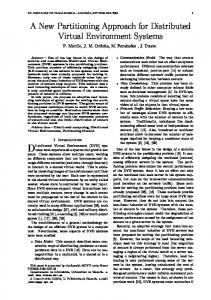
the database is defined as any subset of the transactions contained in the database D. Further, any two different fragments are non-overlapping. Local support for an itemset is the fraction of transactions containing that itemset in a fragment. Local candidate itemset is being tested for minimum support within a given fragment. A Local frequent itemset is an itemset whose local support in the fragment is no less than the minimum support. A Local frequent itemset may or may not be frequent in the context of the entire database. Global support, Global candidate itemset, Global frequent itemset are defined as above except they are in the context of the entire database. The goal is to find all Global frequent itemsets. Firstly, the Partition algorithm divides D into n fragments, and processes one fragment in the main memory at a time. The algorithm first scans fragment Pi, for i = 1,…,n, to find the set of all Local frequent itemsets in Pi, denoted as LPi. Then, by taking the union of LPi, a set of candidate itemsets over D is constructed, denoted as CG (Global candidates). There is an important property: if itemset, X, is a frequent itemset in database D, then X must be a frequent itemset in at least one of the n fragments P1, P2,…, Pn. As a result, CG is a superset of the set of all Global frequent itemsets in D. Secondly, the algorithm scans each fragment for the second time to calculate the support of each itemset in CG and to find which candidate itemsets are really frequent itemsets in D (Figure 3.1). Phase 2

Phase 1 P1

P2

Pn

P1

LP1

LP2

LPn

C

G

P2

Global FI

Pn

data sets in order to partition the original data set more suitably for further processing. In our previous work (Nguyen, Orlowska (2005)), we demonstrated that looking more closely into the data itself may deliver good gains in overall performance. We show how to reach a better data partition based on the relative similarity between the transactions forming the data set. As a result, the number of Local frequent itemsets can be dramatically reduced. Furthermore, in many cases that leads to a larger number of common Global candidates among fragments. Finally, as a consequence, these methods reduce substantially the CG set which must be checked in the Partition algorithm.

4

Data set pre-processing methods

The data set pre-processing is used to partition the input data set in order to get the special fragments which can generate the smaller number of Local frequent itemsets as well as the smaller number of Global candidate itemsets. The goal is to generate the fragments which have more dissimilar transactions. We start with simple illustrations.

4.1

Intuitive example

A giving data set D has only 12 transactions as in table 4.1. Like many other authors in this area, we assume that the set of transactions is ordered by items ids. TID

3.2

Related work

One of the Partition algorithm derivatives is AS-CPA (Anti-Skew Counting Partition Algorithm) by Lin, Dunham (1998). It makes use of the cumulative count of each candidate itemset to achieve a smaller number of Global candidates. The main difference is that AS-CPA provides several effective techniques (Early Local Pruning, Global Anti-Skew) to filter out false candidate itemsets at an earlier stage. Recently, there has been another development based on the partitioning approach in the ARMOR algorithm by Pudi, Haritsa (2003). It uses the array and graph structure to store the cumulative CG while processing the fragments. All the above algorithms mainly attempt to reduce the number of false candidates as early as possible. However, they do not consider any features and characteristics of

TID

List of Items

T1

1,4,12,32

T7

3,6,13,22

T2

1,4,13,30

T8

3,6,14,24

T3

1,4,13,34

T9

3,6,14,22

T4

1,4,13,34

T10

3,6,14,19

T5

1,4,13,36

T11

3,6,17,29

T6

1,4,12,30

T12

3,6,18,23

Table 4.1: Example data set

Figure 3.1: The Partitioning approach

The main goal of this division of process into Local and later Global computation is to process one fragment in the main memory at a time - to avoid multiple scans over D from secondary storage.

List of Items

We assume further, the minimum support threshold at percentage: 50%. After a simple calculation we get; Global frequent itemsets = {{1}, {4}, {3}, {6}, {1,4}, {3,6}} and there are 6 itemsets. The following subsections show clearly how much benefit can be gained by different fragmentations. 4.1.1 Data set partitioned into 2 fragments We consider two different partitions on the same data set to illustrate the dependency of the fragmentation’s composition on the computational cost of the final phase of the Partitioning algorithm. Let D be partitioned into 2 sequent fragments: P1 = {T1, T2, T3, T4, T5, T6} and P2 = {T7,T8,T9,T10, T11, T12}. As a result: LP1 = {{1},{4},{13},{1,4},{1,13},{4,13},{1,4,13}}; |LP1| = 7 LP2 = {{3},{6},{14},{3,6},{3,14},{6,14},{3,6,14}}; |LP2| = 7

CG = LP1 ∪ LP2. Therefore, the number of the Global Candidates, |CG| = 14. Note that there is no common candidate among LPi.

However, if D is partitioned differently into 2 ‘skipping’ fragments such that each fragment holds more dissimilar transactions: P1 = {T1, T2, T3, T7, T8, T9} and P2 = {T4, T5, T6, T10, T11, T12}. As a result: LP1= {{1}, {4}, {13}, {3}, {6}, {1,4}, {3, 6}}; |LP1| = 7 LP2= {{1}, {4}, {3}, {6}, {1,4}, {3,6}}; |LP2| = 6

CG = LP1 ∪ LP2. Therefore, the number of the Global Candidates, |CG| = 7. Note that there are 6 common candidates among LPi, thus only 1 candidate has to be checked in second phase. 4.1.2 Data set partitioned into 3 fragments This example illustrates the relationship between densities of the fragmentation when applied with the expected computation cost. If D is partitioned into 3 sequent fragments: P1 = {T1, T2, T3, T4}; P2 = {T5,T6,T7, T8}; P3 = {T9, T10, T11, T12}. As a result, the number of the Global candidates is |CG| = 22 and there is no common candidate. However, if D is partitioned into 3 ‘skipping’ fragments that have more dissimilar transactions: P1 = {T1, T4, T7, T10}; P2 = {T2, T5, T8, T11}; P3 = {T3, T6, T9, T12}. As a result, the number of the Global candidates is |CG| = 10 and there are 6 common candidates, thus only 4 candidates have to be checked in the second phase of the Partition algorithm. This simple example confirms the fact that there are some relationships between the composition of fragments and the amount of computation required at the end. Our goal is to reduce the cost of this computation.

4.2

The incremental clustering algorithm

The original incremental clustering algorithm was proposed by Nguyen, Orlowska (2005). The requirements for a clustering algorithm restrict the number of scans of the data set. The data set will be scanned only once and all clusters (fragments) containing mostly dissimilar transactions are generated at the end of that scan. The following are some basic definitions. Definition 4.1: Cluster centroid is a set of all items in the cluster, we denote it Ci = {I1, I2,.., In}. Additionally, each item in Ci has its associated weight which is its number of occurrences in the cluster; {w1, w2, …, wn} Definition 4.2: Similarity function between two item sets, in particular a transaction and a cluster centroid, is denoted Sim (Ti, Cj) and defined as follows; Sim (Ti, Cj)

R+ ; Calculation of this function:

1. Let S be the intersection between the arguments of Sim function, S = Ti Cj 2. If S = O / then Sim (Ti, Cj) = 0. Otherwise, S = {I1, I2, …, Im} with the corresponding weights {w1, w2, …, wm} in cluster Cj, respectively, therefore Sim (Ti, Cj) = w1 + w2 + … + wm

Cluster Construction: Informally, each transaction is evaluated in terms of the following criteria; a) We assign a new transaction Ti to cluster Cj which has the minimum Sim(Ti, Cj) value among open clusters (a cluster is open if has not exceeded its expected size in terms of number of transactions). b) Each new allocation to a cluster Cj, updates the cluster centroid Cj. In fact the update can be summarized by the statement; all already existing common items’ weight is increased by 1, and the other new items are added to Cj with the weight of value 1. Reasoning about the size of clusters: the cluster sizes will be well balanced in order to control the number of Local frequent itemsets (LPi). If the size of the cluster is too small, then the number of LPi can be very big mainly due to the fact that the minimum occurrence number of Local frequent itemsets is small. The pseudo incremental clustering algorithm is described as follows. Algorithm 1 (clustering by incremental processing): Input: Transaction database: D; k – number of output clusters Output: k clusters based on the above criteria for Partition approach. Begin 1. Assign the first k transactions to all k clusters, and initialize the all cluster centroids: {C1, C2, …, Ck} 2. Consider the next k transactions. These k transactions are assigned to k different clusters. These operations are done based on the following criteria: (i) the minimum similarity between the new transaction and the suitable clusters; (ii) the sizes of these clusters are controlled to keep the balance. The following are more detail about this processing. Let Crun = {C1, C2, …, Ck } is a set of all k clusters; Trun = {T1, T2, …, Tk } is a set of all k transactions For each transaction Ti in Trun : T1 to Tk Begin a) Calculate the similarity functions between Ti and all the clusters in Crun ; determine the minimum similarity function value, denoted Sim(Ti, Cj) b) Assign Ti to cluster Cj which has the minimum Sim(Ti, Cj) value. Update the cluster centroid Cj c) Remove Cj from the set of all the suitable clusters in order to keep the same size constraint. That means the next transaction is belonged to the existing clusters after removing Cj: Crun = Crun – { Cj}; End Repeat step 2 till all transactions in D are clustered

3. End The time complexity of this incremental clustering algorithm is O(|D| * k *m) where |D| is the number of all transactions, k is the given number of clusters, and m is the number of all items in D.

4.3

Similarity function based on the minimum support threshold

Based on the proposed Algorithm 1, we want to develop new algorithms for further improvements. The similarity function is one of the key points for clustering algorithms. Traditionally, the similarity between two objects is often determined by their bag intersection, the more elements two objects contain, the more similarity they are considered. There are many different measures in use, for example, let X and Y be two objects, |X| is the number of elements in X, the Jaccard’s coefficient (Ganesan et al. 2003), SimJacc(X,Y), is defined to be: SimJacc(X,Y) =

| X ∩Y | | X ∪Y |

However, in the context of frequent itemsets mining we have to consider not only the common items, but also the number of occurrences of items. Therefore, the new similarity function between a transaction and a cluster centroid is defined by a different way as follows: Given database D and the minimum support threshold min_sup (percentage); k is the number of output clusters. With this method, we assume that the sizes of all output fragments are the same. As a result, the minimum number of occurrences for Local frequent itemset in every fragment can be calculated, denoted as supk supk =

| D | * min_ sup ; where |D| is number of all k

transactions in D. The new similarity function is denoted New_Sim(Ti, Cj) R+ , which can be calculated as below: 1). Let Cjk = { I1, I2, …, Im } ⊆ Cj; where all items in Cjk have the corresponding weights in cluster Cj {w1, w2, …, wm} respectively which are no less than (supk - 1); We only consider these items because they may become new frequent items if the new transaction is added to the cluster (their occurrences will increase by 1). Let Sk be the intersection between a transaction Ti and Cjk; Sk = Ti Cjk 2). If Sk = O / then New_Sim (Ti, Cj) = 0. Otherwise, Sk = {Ik1, Ik2, …, Ikn} with the corresponding weights {wk1, wk2, …, wkn} in cluster Cj. Therefore, New_Sim (Ti, Cj) = wk1 + wk2 + … + wkn The Algorithm2 uses the same cluster construction and method as the Algorithm1, but the similarity function is replaced by New_Sim() function. Algorithm 2 (similarity function based on the minimum support threshold): Input: Transaction database: D; min_sup - minimum support threshold; k – number of output clusters Output: k clusters for Partition approach. Begin: 1. Assign the first k transactions to all k clusters, and initialize the all cluster centroids: {C1, C2, …, Ck}

2.

Consider the next k transactions. These k transactions are assigned to k different clusters. Let Crun = {C1, C2, …, Ck } is a set of all k clusters; Trun = {T1, T2, …, Tk } is a set of all k transactions For each transaction Ti in Trun : T1 to Tk Begin a) Calculate the new similarity function between Ti and all the clusters in Crun ; determine the minimum similarity function value, denoted New_Sim(Ti, Cj) b) Assign Ti to cluster Cj which has the minimum New_Sim(Ti, Cj) value. Update the cluster centroid Cj (maintenance of Cj as the Algorithm1 for further computation). c) Remove Cj from the set of all the suitable clusters in order to keep the same size constraint. Crun = Crun – { Cj}; End 3. Repeat step 2 till all transactions in D are clustered End Remarks: This Algorithm2 can reduce dramatically the computation of similarity function, because cluster centroid Cj contains many items (after steps, it contains almost items in database D), but only some of them have the corresponding weights which are no less than (supk - 1). Therefore, the cost of intersection step for similarity computation is reduced.

4.4

Cluster construction based on flexible sizes

The cluster sizes should be well balanced in order to have the same distribution of items among fragments. However, the other cluster construction can be used to get the flexible size of clusters, we want to compare the output result of flexible clusters with those of the other methods and study how much we can gain with this method. Based on the Algorithm1, this method uses the same similarity function Sim(Ti, Cj). We extend to the new pre-processing algorithm as follows. Algorithm 3 (based on the flexible sizes of clusters): Input: Transaction database: D; k – number of clusters Output: k clusters for Partition approach. Begin 1. Assign the first k transactions to all k clusters, and initialize the all cluster centroids: {C1, C2, …, Ck} 2. Consider the next transaction. This transaction is assigned to cluster which has the minimum similarity between the new transaction and the clusters. Let Crun = {C1, C2, …, Ck } is a set of all k clusters; the new transaction Ti Begin a) Calculate the similarity functions between Ti and all the clusters in Crun ; determine the minimum similarity function value, denoted Sim(Ti, Cj) b) Assign Ti to cluster Cj which has the minimum Sim(Ti, Cj) value. Update the cluster centroid Cj End 3. Repeat step 2 till all transactions in D are clustered End

5

Experimental results

In this section, we conducted experiments on three data sets: one synthetic data set (T10I4D100K) generated by Agrawal, Srikant (1994), one small real data set and one big real data set (BMS-WebView-1 and BMS-POS) from Ron et al. (2000). These data sets are converted to format as the above definitions. Data sets

Transactions

Items

DB Size (~MB)

T10I4D100K

100K

870

4

WebView-1

26K

492

0.7

BMS-POS

435K

1657

10

Table 5.1: The characteristics of data sets Our goal is to compare the cardinality of the outputs; at the Local level and the Global level, before and after application of our pre-processing methods. The expectation is that the final computation cost of Partition algorithm reduces dramatically after pre-processing. Firstly, data set is partitioned into fragments; secondly the Apriori algorithm implemented by Zhu T. (2004) is applied to find Local frequent itemsets (LPi) for each fragment. Subsequently, union of these LPi generates the Global candidates. Resulting figures for each data set are represented in following template table 5.2. The 2nd, 3rd, 4th and 5th columns’ names indicate four methods for data preparation: Sequent fragments correspond to loading clusters with original data (no pre-processing), Clustering fragments are constructed as described in section 4.2 (Algorithm1); the New similarity function fragments are the other pre-processed data as presented by our new method described in section 4.3 (Algorithm2); the New cluster construction fragments are the other new method described in section 4.4 (Algorithm3).

Algorithm2 with the threshold 0.01 for real data set WebView-1, and its value reduces from 1,820 for Sequent to 756 for Algorithm2 with the threshold 0.005 for very large data set BMS-POS. Moreover, if data sets are partitioned into 5 fragments, the gap is even greater. For example, if T10I4D100K is partitioned into 5 fragments, |C5G| decreases from 48 for Sequent to 24 for Algorithm1 with the threshold 0.01. |C5G| decreases from 698 for Sequent to 434 for Algorithm3 with the threshold 0.005. When WebView-1 is partitioned into 5 fragments, |C5G| decreases from 425 for Sequent to 93 for Algorithm2 with the threshold 0.01. Exceptional performance for BMS-POS when data set is partitioned into 5 fragments for Algorithm2: with the threshold 0.01 the reduction is from 2,263 to only 222 as well as with the threshold 0.005 it reduces significantly from 10,718 to only 1,192. Secondly, another interesting and encouraging trend can be found in the growth of the number of common candidates between LPi for fragmented data sets. For example, if data sets are partitioned into 2 fragments, this common number increases from 152 to 203 for Algorithm1 with WebView-1 and the threshold 0.01. In addition, if data sets are partitioned into 5 fragments, this common number increases dramatically from 689 to 1,404 for Algorithm2 with BMS-POS and the threshold 0.01 as well as from 2,346 to 4,563 for Algorithm3 with the same data set and the threshold 0.005.

Further, to discuss the impact of different fragmentations and threshold level, let us denote the cardinality of checked Global candidates set as |CnG|, where n is the number of fragments. As can be seen from table 5.2 and table 5.3, there are big gains from the careful data preprocessing methods.

For comparison, we can compare these three preprocessing methods (Agorithm1, Agorithm2, Agorithm3) based upon several metrics. Firstly, the number of Global candidates of Algorithm1 is less than those of the others for almost data sets and minimum support thresholds. In contrast, Agorithm3 has the highest number of Global candidates for all data sets and all minimum support thresholds. Because there are different sizes of output clusters of Agorithm3, so the Local frequent itemsets of clusters are more different and the number of them is higher. As a result, the number of Global candidates is higher. For Agorithm2, with very big real data set (BMSPOS) and the higher number of fragments (5 fragments), the output result is more benefit than those of the other methods. For example, the numbers of Global candidates are 222 with threshold 0.01 and 1,192 with threshold 0.005 in comparison with those of Agorithm1 are 894 and 4,075, respectively. Secondly, as mentioned in section 4.3, Agorithm2 can save much more computation of the similarity function that the other methods. This is very efficient when the data sets have many different items. Consequently, the better methods can be selected depending on the characteristics of data sets such as the number of all items, the number of all transactions and the given minimum support threshold.

Firstly, |CnG| is reduced for all data sets for all minimum support thresholds. For example, if T10I4D100K is partitioned into 2 fragments, |C2G| decreases from 16 for Sequent to 4 for Algorithm3 with the support threshold 0.01. This reduction is also present when considering other real data sets that are partitioned into 2 fragments. Its value reduces from 152 for Sequent to 46 for

In summary, the figures from two tables show that the all data pre-processing methods can significantly improve the Partitioning approach. It is delivered in form of two strongly related benefits; reduction of the number of Global candidates requiring the final check and increase of the common candidates numbers that don’t require any additional checks.

The data sets used are indicated on the top of each table segment. We present three different scenarios; each data set is partitioned into 1, 2 and 5 fragments. Each column represents the numbers of the Local level (LP1, LP2, …, LPn), the number of Global candidates. Note that this figure is presented by showing its two components; for example; it, 16 + (378), indicates that there are 16 candidates to be checked and 378 common candidates don’t need additional check.

Sequent

Clustering

(no processing)

(Algorithm1)

New similar Function

New Construction

(Algorithm2)

(Algorithm3)

Sequent

Clustering

(no processing)

(Algorithm1)

T10I4D100K

New Similar Function

New Construction

(Algorithm2)

(Algorithm3)

T10I4D100K

1-fragment: 385 Frequent Itemsets

1-fragment: 1,073 Frequent Itemsets

2 fragments

2 fragments

LP1

385

385

383

385

LP1

1,079

1,068

1099

1091

LP2

387

386

391

389

LP2

1,101

1,092

1084

1079

4 + (385)

C2G

158 + (1,011)

70 + (1,045)

213 + (985)

88 + (1041)

C2G

16+ (378)

3 + (384)

12 + (381)

5 fragments

5 fragments

LP1

392

387

391

383

LP1

1,150

1,089

1087

1040

LP2

381

387

394

385

LP2

1,141

1,110

1088

1032

LP3

393

384

390

388

LP3

1,248

1,059

1092

1111

LP4

386

388

395

391

LP4

1,110

1,135

1094

1161

LP5

390

388

391

393

LP5

1,120

1,098

1136

1150

33 + (381)

C5G

698 + (893)

373 + (941)

268 + (976)

434 + (960)

C5G

48+ (366)

24+ (375)

31 + (379)

WebView-1

WebView-1

1-fragment: 208 Frequent Itemsets

1-fragment: 633 Frequent Itemsets

LP1

227

210

196

184

LP1

644

659

581

529

LP2

229

213

232

262

LP2

755

641

744

859

78 + (184)

C2G

503 + (448)

94 + (603)

191 + (567)

330 + (529)

C2G

152+ (152)

17+ (203)

46 + (191)

5 fragments

5 fragments

LP1

284

226

220

154

LP1

1,107

779

766

413

LP2

197

221

212

186

LP2

489

733

722

552

LP3

241

213

228

231

LP3

839

676

751

770

LP4

255

207

228

270

LP4

894

663

648

898

LP5

266

205

216

353

LP5

977

597

615

1601

C5G

425+ (92)

74+ (181)

93 + (182)

311 + (154)

C5G

1,806 + (271)

497 + (493)

538 + (485)

1643 + (404)

BMS-POS

BMS-POS

1-fragment: 1,503 Frequent Itemsets

1-fragment: 6,017 Frequent Itemsets

LP1

1,400

1,512

1,348

1,378

LP1

5,419

6,024

5,699

5,502

LP2

1,662

1,498

1,688

1,655

LP2

6,709

5,972

6,385

6,559

277 + (1,378)

C2G

1,820+ (5,154)

348+ (5,824)

756 + (5,664)

1,061 + (5,500)

C2G

390+ (1,336)

60+ (1,475)

342 + (1,347)

5 fragments

5 fragments

LP1

1,996

1,150

1536

1,192

LP1

8,480

4,339

6,023

4,586

LP2

1,334

1,471

1505

1,359

LP2

4,975

5,932

5,894

5,395

LP3

744

1,864

1514

1,576

LP3

2,541

7,530

6,163

6,313

LP4

1,348

1,822

1474

1,700

LP4

5,177

7,443

6,017

6,835

LP5

2,885

1,364

1521

1,858

LP5

12,755

5,289

6,109

7,473

1,356 + (1,192)

C5G

10,718+ (2,346)

4,075+ (4,191)

1,192 + (5,467)

6,029 + (4,563)

C5G

2,263+ (689)

894+ (1,121)

222 + (1,404)

Table 5.2: The figures with a support threshold 0.01

Table 5.3: The figures with a support threshold 0.005

6

Conclusion

As an extension of our previous work, this paper considers the extension of data pre-processing approach for further performance improvements in frequent itemsets computation. We show that the composition of fragments and the number of fragments generated, impact on the size of the data used by the original Partition algorithm. We proposed a series of data pre-processing methods, mainly to demonstrate that the performance of computing frequent itemsets can be improved by data partitioning. The new algorithms are proposed based on different definitions of similarity function and different cluster constructions which are applied for data clustering to get more efficient. Figures from the experiments show that these data pre-processing methods offer good benefits already. In addition, the comparison among these methods has been conducted. In particular, the better method can be applied depending on the characteristics of input data sets and the given minimum support threshold. There is an interesting question for future work which is how to identify the methods that will deliver an even better partition for the original data sets.

7

References

Nguyen S., Orlowska M. (2005): Improvements in the Data Partitioning Approach for Frequent Itemsets Mining. Proc. 9th European Conference on Principles and Practice of Knowledge Discovery in Databases (PKDD 05), Springer. Agrawal R., Imielinski T., Swami A. (1993): Mining association rules between sets of items in lagre database. Proc. 1993 ACM SIGMOD Int. Conf. on Management of Data, Washington DC, USA, 22:207216, ACM Press. Agrawal R., Srikant R. (1994): Fast algorithms for mining association rules. Proc. 20th Int. Conf. Very Large Data Bases, Morgan Kaufmann, (487 - 499) Brin S., Motwani R., Ullman D.J., Tsur S. (1997): Dynamic Itemset Counting and implication rules for masket basket data. Proc. ACM SIGMOD 1997 Int. Conf. on Management of Data, (255 - 264) Houtsma M., Swami A. (1995): Set-oriented mining for association rules in relational database. Proc. 11th IEEE Int. Conf. on Data Engineering, Taipei - Taiwan, (25 - 34) Lin J.L., Dunham M.H. (1998): Mining association rules: Anti-skew algorithms. Proc. 14th IEEE Int. Conf. on Data Engineering, Florida Pudi V., Haritsa J. (2003): ARMOR: Association rule mining based on Oracle. Workshop on Frequent Itemset Mining Implementations (FIMI'03 in conjunction with ICDM’03)

Savasere A., Omiecinski E., Navathe S. (1995): An efficiant algorithms for mining association rules in large database. Proc. 21th Int. Conf. Very Large Data Bases, Swizerland Toivoven H. (1996): Sampling Large Databases for association rules. Proc. 22th Int. Conf. Very Large Data Bases, Mumbai, India Ron K., Carla B., Brian F., Llew M., Zijian Z. (2000) KDD-Cup 2000 organizers' report: Peeling the onion. SIGKDD Explorations, 2(2):86-98 Goethals B. (2002): Survey on frequent pattern mining. University of Helsinki Mueller A. (1995): Fast sequential and parallel algorithm for association rules mining: A comparision. Technical Report CS-TR-3515, Uni. of Maryland Zhu T. (2004): The Apriori algorithm implementation, http://www.cs.ualberta.ca/~tszhu/, Accessed 2004 Han J., Pei J., Yin Y., Mao R. (2004): Mining frequent patterns without candidate generation: A frequentpattern tree approach. Data Mining and Knowledge Discovery, Kluwer Academic Publishers, (8): 53-87 Zaki M.J. (2000): Scalable algorithms for association mining. IEEE Transactions on Knowledge and Data Engineering, 12(3): 372-390 Zhang S., Wu X. (2001): Large scale data mining based on data partitioning. Applied Artificial Intelligence 15:129-139 Ganesan P., Garcia-Monila H., Widom J. (2003): Exploiting hierarchical domain structure to compute similarity. ACM Transactions on Information systems. Vol. 21, No. 1, January 2003.