Author’s version of article in Integrated Computer-Aided Engineering, 19(3):257-271, 2012, IOS Press. doi:10.3233/ICA-2012-0405
A generalization of quad-trees applied to image coding Rade Kutil Department of Computer Sciences, University of Salzburg, Jakob Haringer-Str. 2, 5020 Salzburg, Austria E-mail:
[email protected]
Abstract.Although quad-trees are not the most successful strategy in image coding, some generalized subdivision schemes have been proposed recently. This work exploits a moderate generalization of quad-trees where tiles are not restricted to be split in both dimensions, which leads to a previously developed graph of anisotropic tiles called “bush”. An algorithm is developed to find the minimal number of tiles to represent shapes, which is used to build a codec for bi-level and indexed color images. Also, a lossy codec based on tile-wise rate-distortion optimized quantization of low-frequency DCT coefficients is developed. The aim of this work is to investigate whether anisotropic tiles have an advantage over square tiles. The results indeed show significant improvements. The lossless algorithm is suitable for images with large continuous regions and high color payload, such as geographical maps. The lossy codec is able to compete with JPEG2000, especially for artificial images.
Keywords: image coding, quad-tree, DCT, rate-distortion
1.
Introduction
Quad-trees have long been used in general image coding [34], for bi-level images [23], cartoon images [38], and video coding [20]. In quad-tree coding, square tiles are recursively decomposed into four square subtiles. The process stops for sufficiently uniform tiles, for which the color payload is encoded. The tree structure also has to be encoded. However, the advantage of quad-trees is that they can be encoded efficiently by only one bit per tile that indicates if it is split or not. For bi-level or indexed color images, the payload is the pixel color. For natural images, image segments are approximated by planar [22, 31] or polynomial [27, 32] functions. Generalized tilings with arbitrarily oriented linear splitting are used here, though, to achieve a more accurate approximation of region borders. However, this leads to increased bit budgets for encoding of the segmentation structure, so block merge algorithms [42] or combinations with quadtrees [12] have been developed. These schemes can be applied to DCT [19] and wavelet [39] coding, as well as motion estimation [2, 28, 44] in video coding. Common to these applications is the amount of data to be encoded per tile, which is larger than the single bit payload for bi-level
images, where JBIG2 [25] or chain codes [30] are far superior. Another reason to use tree structures to encode image data is the ability to arbitrarily select spatial details, as needed in terrain visualization [3] and display of geospatial data [45]. Also, spatial databases use quad-trees [13] in a similar way. Apart from that, [1, 4–11, 24, 26, 35] are somewhat related to the topic. This work exploits a moderate generalization of quad-trees. It admits non-square tiles, but does not go as far as generalized tilings at arbitrary positions and angles. Thus, it retains some of the economical encodability of quad-trees while offering a somewhat greater flexibility. Tiles may be split anisotropically in horizontal or vertical dimension, which may produce highly non-square tiles. The number of these decompositions was shown to be much higher than that of quad-trees [16, 43]. Moreover, the representation as a binary tree of horizontal or vertical splits is not unique, and, therefore, causes redundancy and inefficiency in coding. However, if the graph structure is expanded to incorporate all possible decomposition trees with the same set of leaf nodes, uniqueness is achieved. In [14–16], such a graph, called “bush”, together with an efficient redundancy-free coding algorithm has been developed. Redundancy-free means that there is only one representation for each set of
tilings and, when encoded, no encoded symbol can be deduced from other parts of encoded data. An efficient coding algorithm is important in our context because the amount of data necessary to represent the tiling structure is not negligible compared to the coding of color payload. In this work, an algorithm to find the best bush tiling for an image, in terms of tile count, is presented, and a lossless coding scheme for the color information is developed. The coding scheme aims at images with large uniform areas which may occur in geographical maps or technical drawings. A class of images is generated by randomly growing blots, optionally followed by smoothing operations, to test the coding efficiency and to compare it to JBIG2 and PNG. The aim is to investigate, what the benefits of bush tilings are over conventional quad-tree tilings, and which kind of image data they are suitable for. This first part can also be found in [17]. In the second part of this work, based on these insights, a new lossy image compression algorithm is developed in order to demonstrate the benefits of bush tilings on general images. It applies successive bitplane coding of a subset of low-frequency DCT coefficients, which are calculated for each tile. These DCT coefficients are considered as a tile-wise approximation in the sense of piece-wise planar or polynomial approximations as in [27, 32]. The bit-rate per tile is controlled by the number of bitplane passes performed. The optimal number of passes for each tile is determined by rate-distortion optimization. The best tiling is also found in terms of this rate-distortion optimization by minimizing the sum of rate-distortion values, which leads to a variant of the optimal tiling algorithm of the lossless case. The schemes are compared to JPEG2000. Section 2 presents the algorithm to find tilings with a minimal number of anisotropic tiles. Section 3 develops the lossless coding algorithm for shapes represented by an optimal tiling. In Section 4, the set of test shape images is generated. Results for the lossless case are shown in Section 5. Section 6 develops the lossy coding algorithm, and Section 7 presents the coding performance results. Section 8 concludes the findings of this work. 2.
Tiling algorithm
Anisotropic tilings lead to non-unique decompositions in terms of binary trees. See e.g. Figure 1, where four square sub-tiles can be produced either by hori-
Figure 1: A full bush of anisotropic tiles
(a) shape
(b) quad-tree
(c) bush
Figure 2: A shape and its decomposition into 3514 quad-tree tiles and 1861 bush tiles.
zontal followed by vertical splitting, as well as in the reverse order. The coding of such a decomposition tree is, therefore, necessarily redundant. By incorporating all decomposition trees into a two-dimensional graph structure, called “bush”, a unique representation is achieved. This graph is basically a Cartesian product of two binary trees, or a subgraph thereof. It is not a tree because it contains cycles. The condition that the bush must contain all possible decomposition trees can be checked and enforced in a local fashion by inheriting complete splits up and down the hierarchy of nodes. This allows to encode splits as early as possible in a top-down coding scheme and to omit redundant split information at deeper levels in the graph. For an efficient coding algorithm of bushes, see [14–16]. It basically encodes whether a tile is split horizontally, vertically or both. Then it passes the information about the vertical split to horizontal child tiles, or vice versa. If that information indicates a vertical split, the horizontal child also has to be split vertically, so this does not have to be encoded. If the information indicates no split, the only one horizontal child may be split, which also reduces the information to be encoded. This is repeated recursively. The results is a unique bitstream that is free of redundancy. However, there are still several possible bush tilings for a given shape, contrary to quad-trees, which are always unique. As these bush tilings have different numbers of tiles, we want to find the one with the lowest number of tiles. See Figure 2 for an example. First,
5 4 3 2 3 3 3
(a) shape
1 1 1 1 1 1 1
4 3 2 1 2 2 2
1 1 1 1 1 1 1
1 1 1 1 1 1 1
3 2 1 1 1 1 1
(b) algorithm
1 1 1 1 1 1 1
(c) result
Figure 3: Example for optimal tiling algorithm
we need a way to arrange all possible tiles of an image. Since a bush is a product of two binary trees, and a binary tree can be arranged as a 1-D array, bush-nodes can be arranged in a 2-D array of size 2m−1×2n−1, where m × n is the image size, and m and n are, for simplicity, a power of two. See Figure 3 for an example. The right lower m × n-block of this array is filled with image data. Each node is associated with the best number of tilings it can be decomposed into. This number is calculated from the lower right to the upper left corner. If a tile is uniform, it gets a 1. Otherwise, it gets the minimum of the sum of the horizontal or vertical sub-tiles, and is associated with the corresponding decomposition dimension. In the end, the upper left node contains the minimum number of tiles for the image. Following the optimal decomposition dimensions, starting from the upper left node, the optimal bush can be created. Figure 4 shows the actual algorithm. In the first double loop, the arrays are initiated for pixel-size leaf nodes in the region {2k − 1, . . . , 2(2k − 1)} × {2l − 1, . . . , 2(2l − 1)}, where the subtile count n[i0 , j 0 ] is 1, the split dimension d[i0 , j 0 ] is u for “no split”, and c[i0 , j 0 ] gets the corresponding pixel color. Then a double loop iterates from the bottom-right to the upper-left corner. For each node [i, j], [2i+1, j] and [2i+2, j] are the horizontal child nodes, and [i, 2j +1] and [i, 2j +2] are the vertical child nodes. First, if both child nodes have the same color, then c[i, j] is set to that color and the horizontal minimal subtile count is set to 1. Otherwise, it is set to the sum of the subtile counts of the child tiles n[2i + 1, j] + n[2i + 2, j]. The same is done in the vertical dimension. Then, if the horizontal or vertical minimal subtile count is 1, the optimal split dimension d[i, j] is set to u. Otherwise, it is set to the dimension (h or v) of the smaller subtile count. The bush structure is then built along these optimal split dimensions, beginning with the root node, with the recursive procedure makeTiling.
for i = 0 . . . 2k − 1 // initialize arrays n, d, c for j = 0 . . . 2l − 1 i0 = i + 2k − 1; j 0 = j + 2l − 1 n[i0 , j 0 ] = 1; d[i0 , j 0 ] = u; c[i0 , j 0 ] = I[i, j] for i = 2k+1 − 1 . . . 0 // main algorithm for j = 2l+1 − 1 . . . 0 nh = nv = ∞ if 2i + 2 < 2k if c[2i + 1, j] = c[2i + 2, j] 6= −1 c[i, j] = c[2i + 1, j]; nh = 1 else nh = n[2i + 1, j] + n[2i + 1, j] if 2j + 2 < 2l if c[i, 2j + 1] = c[i, 2j + 2] 6= −1 c[i, j] = c[i, 2j + 1]; nv = 1 else nv = n[i, 2j + 1] + n[i, 2j + 1] if nh = 1 or nv = 1 d[i, j] = u; n[i, j] = 1 else if nh ≤ nv d[i, j] = h; n[i, j] = nh else d[i, j] = v; n[i, j] = nv makeTiling (0, 0, I) // root node is whole image makeTiling (i, j, T ) := // build bush recursively if d[i, j] = h split T horizontally makeTiling (2i + 1, j, left subtile of T ) makeTiling (2i + 2, j, right subtile of T ) if d[i, j] = v split T vertically makeTiling (i, 2j + 1, upper subtile of T ) makeTiling (i, 2j + 2, lower subtile of T ) Figure 4: Pseudo code of tiling algorithm for image I with size 2l × 2k . Array n contains subtile count, c tile color, and d preferred split dimension (h . . . horizontal, v . . . vertical, u . . . uniform/no split).
for T in nodes of bush if T is not leaf choose split dimensions d if first child T1 in dim. d is leaf encode c(T1 ) else if second child T2 of T in dim. d is leaf encode c(T2 )
for T in nodes of quad-tree if T is not leaf if all 4 children T1 , T2 , T3 , T4 of T are leaves encode c(T1 ) + 2c(T2 ) + 4c(T3 ) + 8c(T4 ) − 1 else for i = 1 . . . 4 if Ti is leaf, then encode c(Ti )
Figure 5: Color coding of bi-level image with bushes.
Figure 6: Color coding of bi-level image with quadtrees.
The resulting tiling is optimal in the sense that it uses the smallest number of tiles to represent a given shape. This can be seen from the fact that each nonuniform tile is decomposed into the smallest number of subtiles by splitting it either horizontally or vertically. The smallest number of subtiles is then either given by the smallest number of subtiles the horizontal child tiles can be decomposed into, or by that of the vertical child tiles. The smaller of the two possibilities gives the optimal result for a tile. The recursive application of this principle to all possible tiles guarantees the optimality for the root tile, i.e. the whole image. Image sizes that are not a power of two can be handled easiest by simply expanding the image to powerof-two size and filling the expanded area with the color of nearest margin pixels. In this way, only a slight enlargement of the bush and only a few additional tiles are required. When decoding an image, the expanded area is discarded.
for T in nodes of bush if T is not leaf choose split dimensions d if first child T1 in dim. d is leaf encode whether c(T ) = c(T1 ) if c(T ) 6= c(T1 ) remove c(T ) from arith. coder model encode c(T1 ) c(T ) = c(T1 ) if second child T2 in dim. d is leaf if T1 is not leaf encode whether c(T ) = c(T2 ) if T1 is leaf or c(T ) 6= c(T2 ) remove c(T ) from arith. coder model encode c(T2 ) c(T ) = c(T2 ) if T1 is not leaf, then c(T1 ) = c(T ) if T2 is not leaf, then c(T2 ) = c(T ) Figure 7: Color coding of color image with bushes.
3.
Color coding
After the bush structure is encoded using the algorithm in [14–16], the color information has to be encoded for each leaf tile. For bi-level images, each leaf tile is encoded with one bit (to be more precise, one out of two symbols in the arithmetic coder), except if two sibling tiles are both leaves, in which case only one tile has to be encoded, the other one must have the other color. Figure 5 shows the algorithm. It traverses the nodes of the bush in a depth-first order of a spanning tree. The “else if” line implies that T2 is only encoded if T1 is not also a leaf tile. For quad-trees, a similar scheme is used. See Figure 6. Only for a set of four sub-tiles that are all leaves, a second model is used in the arithmetic coder to encode all sub-tiles together as one out of 14 symbols, since the two combinations of all equal colors are not possible.
For multi-color images, the situation is more complicated. Colors that appear at one point in a sub-tree or sub-bush are more probable than other colors to appear in other nodes in the same sub-tree or sub-bush. Therefore, when a leaf-node is encoded, its color is passed on to its parent node and to all child nodes of the latter. See Figure 7 for the bush case, and Figure 8 for the quad-tree case. Before encoding a leaf-node’s color, the information is encoded whether its color is equal to the color passed on from its parent node. The color only has to be encoded if a “no” has been encoded, and the passed-on color is removed from the arithmetic coder’s model. In the case of sibling leaf nodes, “no” can be assumed without coding for the second node (in the bush case) or the last node (in the quad-tree case when the first three nodes have equal color) because these nodes must have a color that is
for T in nodes of quad-tree if T is not leaf for Ti in children T1 , T2 , T3 , T4 of T if Ti is leaf e =false if not (i = 4 and T1 , T2 , T3 leaves and c(T1 ) = c(T2 ) = c(T3 )) encode whether c(Ti ) = c(T ) if c(Ti ) = c(T ) then e =true; if not e remove c(T ) from arith. coder model encode c(T ) c(T ) = c(Ti ) for Ti in T1 , T2 , T3 , T4 if Ti is not leaf then c(Ti ) = c(T ) Figure 8: Color coding of color image with quad-trees.
(a) raw
(b) smoothed
(c) aligned
(d) colors
Figure 9: Generated shapes made of 40 blots. (a) has 3.9% border pixels, (b) is smoothed with a 33 × 33filter to 2.4% border pixels, (c) is aligned with a 65 × 5-filter to 1.17% aligned and 1.07% diagonal border pixels, (d) has 16 colors with one blot for each color. different from the color that is passed on from the sibling nodes. 4.
in four directions are inserted into the buffer. Pixels that are already colored are discarded. The process stops when the buffer is empty. See Figure 9 (a) for an example. Because the result has very ragged borders, an optional smoothing filter is applied. It takes the form of a block centered around each pixel. The pixel’s color is substituted by the most frequent color in that block. The larger the block, the smoother the result will be. See Figure 9 (b) for an example. To quantify the smoothness of the result, all (overlapping) 2 × 2-blocks of the image are classified as either mono-colored or, otherwise, as border blocks. The rate of border blocks approximates the rate of border pixels. A border pixel is a pixel that is located at the border of a uniform region. The border pixel rate is determined by the number of blot seeds, the number of colors, and the smoothing block size. The bit-rate of compressed images is expected to grow linearly with this rate because the information content of a shape is contained in its border. The more complex a shape is, the longer will be its border. Therefore, the number of border pixels is a better measure of image content than its size. Moreover, anisotropic bush tilings prefer horizontally or vertically aligned borders for obvious reasons. To achieve such an alignment, the filter block is modified to have a cross shape made of two rectangular blocks of size a × b and b × a respectively. See Figure 9 (c) for an example of a filtered image. To quantify also the alignment of blot borders, we further classify border blocks into diagonal blocks if two diagonal pixels are equal, and aligned blocks otherwise. The difference between aligned and diagonal pixel rates is a measure for the overall horizontal and vertical alignment of the blot borders.
Test image generation 5.
The lossless coding algorithm is certainly not applicable to natural images because it relies on areas of constant color. Bi-level versions of natural images with dithering also do not meet this condition. So the target application is shape coding. Therefore, we want to generate a set of test images with a certain range of properties. They should contain areas of constant color with arbitrary borders, similar to geographical maps. This is done by randomly growing blots. For each color, a certain number of pixel seeds are placed on the image and stored in a buffer of border pixel positions. Buffer entries are randomly chosen, and, after coloring the corresponding pixel, their neighbors
Results for lossless coding
A total of 745 bi-level images and 1292 colored images of size 1024 × 1024 have been generated to test the performance of our quad-tree and bush coding schemes. Figure 10 shows overall results depending on the rate of border pixels for bi-level images. As the bit-rate is expected to grow linearly with this rate, it is not calculated in bits per image pixel but in bits per border pixel, so that a constant curve indicates a linearly growing bit-rate. Individual results are grouped into bins of equal number of images, and the average bit-rate together with error bars representing the standard deviation are shown. JBIG2 is superior and PNG
PNG quadtree bush jbig2
7 6
tiles per border pixel
bits per border pixel
8
5 4 3 2 1 0.1
0.2
0.5 1 border pixels in percent
2
Figure 10: Bit-rate depending on the number of pixels lying at region borders
6
graph bits in percent
7
PNG quadtree bush jbig2
5 4 3 2 1 -0.2
-0.15
-0.1 -0.05 0 0.05 0.1 aligned minus diagonal pixels in percent
0.15
is inferior compared to our coding schemes. Note that all schemes exhibit a linear growth of bit-rate with the border pixel rate, except for PNG, which cannot benefit as much from larger blots of constant color. Note that bush tilings do not necessarily have better performance than quad-tree tilings because the encoding of the bush graph needs more bits than a quadtree. In this case, quad-tree and bush tilings show approximately equal performance for general bi-level images. However, bush tilings have much larger deviation. This indicates that there are some images where bush tilings perform significantly better, and others where they are worse. It turns out that the border alignment is what causes this phenomenon. Figure 11 shows that the bit-rate drops by almost one bit per border pixel for images with more aligned than diagonal pixels. This is of importance because many images naturally incorporate horizontal and vertical features. The reason for this behavior is the reduced number of anisotropic tiles for such images, as can be seen in Figure 12. This figure also shows that bush tilings are able to reduce the number of tiles by approximately two for all images. Accordingly, the bit-rate used for encod-
-0.3
-0.2 -0.1 0 0.1 0.2 0.3 aligned minus diagonal pixels in percent
80 70 60 50 40 30 20 10 0
0.4
quadtree bush
2
0.2
Figure 11: Bit-rate depending on the degree of alignment (horizontal and vertical) of region borders
quadtree bush
Figure 12: Number of tiles depending on the degree of alignment of region borders
4
8
16 32 number of colors
64
128
256
Figure 13: Share of bits used to encode the graph structure
bits per border pixel
bits per border pixel
8
2.2 2 1.8 1.6 1.4 1.2 1 0.8 0.6 -0.4
11 10 9 8 7 6 5 4 3
PNG quadtree bush
4
8
16 32 64 number of colors
128
256
Figure 14: Bit-rate depending on the payload, i.e. number of colors, for border pixel rates between 3 and 4 ing the graph structure is much higher for bush tilings than for quad-tree tilings, as can be seen in Figure 13. Conversely, the bit-rate for color information is much lower, due to the reduced number of tiles. This effect even grows with the number of colors because the bitrate for color coding becomes more prominent. As a result, a higher number of colors increases the competitiveness of bush tilings, as can be seen in Figure 14. Bush tilings are clearly superior to quad-trees, and the quotient of their bit-rates evolves in favor of bush tilings while the number of colors grows. Note
that the border pixel rate is quite high in Figure 14 in order to fit 256 blots into the image. This is the reason that PNG is able to beat bush tilings for images with over 40 colors. For larger images, blots are also larger, and PNG performs far worse, as shown in Figure 10. Note also that the bit-rate for PNG remains about constant in Figure 14 while that of quad-tree and bush tilings increases linearly. This shows that the bit budget for representing shapes is prominent in PNG while the pure color information is comparably negligible. 6.
Lossy image coding
Insights from the lossless algorithm tell us that bush tilings will enable more efficient compression than quad-tree tilings in case of big color payloads per tile. Schemes like piece-wise linear or polynomial approximations on tiles meet this condition. It is therefore promising to develop such a scheme for anisotropic bush tilings. The result will be suitable for images with smooth areas and sharp borders, as can be found in technical drawings, screenshots or cartoons. In order to use tilings in lossy image coding, we need a reasonable coding algorithm that is applicable to rectangular tiles. Each tile should represent a good local image approximation. Refinements on the approximation shall not be achieved by a more detailed description of the contents of a tile, but by splitting a tile into smaller ones that can be approximated more easily. Therefore, we perform a discrete two-dimensional cosine transform (DCT) on the tiles and select a subset of the coefficients as the approximation of the tile’s content. The subset chosen is, of course, a set of lowfrequency coefficients. It is organized as a number of slots. Each slot groups coefficients with horizontal frequency index i and vertical index j so that i + j is the slot’s index. See Figure 15 (a). Slot 0 contains the so-called DC coefficient. When n slots are used, then n(n + 1)/2 coefficients are to be encoded, all others are neglected. If other coefficients contain too much energy, so that the approximation error is too big, then the tile has to be split. The choice of DCT is, of course, motivated by JPEG, but also by [19] which uses DCT on quad-tree tilings. The shape of the slots is motivated by the zig-zag scan order of JPEG. To encode the DCT coefficients efficiently, we apply a bitplane approach, as is usual in modern compression schemes [36, 37, 46]. Beginning with a maximum threshold, the most significant bits of the DCT
sign significance refinement
0 1 2
3
+ 101 + - 10 + 11 -
101 110 011 100
0 0 0 1 1
0 1 0 0 1
1 0 1 0 0
sig. change no change
(a) slots
(b) bitplanes
(c) sig. context
Figure 15: coding of DCT coefficients
coefficients are encoded so that the quantization error of each coefficient is smaller than the threshold. The quantization is then refined in subsequent passes with the threshold being divided by two in each pass. DC coefficients tend to dominate the energy in the tile’s DCT domain. This problem is somewhat relieved by simply subtracting the average of the whole image from the image, which has to be encoded in the beginning. Figure 16 shows the algorithm. For each coding pass, it first checks whether there are insignificant coefficients (˜ c[i, j] = 0) that become significant in that pass (|c[i, j]| ≥ 2k ), which is encoded. Thus, a pass with no changes in coefficient significance is abbreviated by a single bit for the whole pass. It then iterates through the set P of coefficient indices. For insignificant coefficients, their new significance is encoded, and, if significant, its sign bit has to be encoded as well. For significant coefficients, a refinement bit is encoded. Arithmetic coding is used to encode significance bits, refinement bits and sign bits of the DCT coefficients. See Figure 15 (b). Refinement and sign bits have a 50% percent probability for 1 and 0. Significance bits, however, correlate with those of neighboring coefficients. Therefore, they are classified into two contexts depending on whether the left or upper neighbor, i.e. (i − 1, j) and (i, j − 1), was significant in a previous pass. See Figure 15 (c). When those two neighbors are not significant, then there is a chance of only 10% or lower that the coefficient becomes significant. Otherwise, the probability is higher, i.e. about 50% for more than 3 slots, 40% for 3 slots, and 30% for 2 slots. These probabilities are used in a fixed way in the arithmetic coder, no adaptivity is applied. This has the advantage of better computational performance and, more important, the rate-distortion analysis is exact because bit statistics of neighboring tiles have no influence on the bit-rate.
c . . . DCT transform coefficients for tile c˜ . . . reconstructed approximation of c; c˜[·, ·] = 0 P = {(i, j) | i, j ≥ 0, i + j < slots}∩ tile range k=8 // maximum bitplane for # coding passes k =k−1 s :⇔ ∃(i, j) ∈ P : 2k ≤ |c[i, j]| < 2k+1 if ∃(i, j) ∈ P : c˜[i, j] = 0 then encode s for (i, j) ∈ P c˜old = c˜[i, j] if c˜[i, j] = 0 if s if i > 0 and |˜ c[i − 1, j]| ≥ 2k+1 or j > 0 and |˜ c[i, j − 1]| ≥ 2k+1 or i = j = 0 if slots = 2 then f1 = 3; f0 = 7 else if slots = 3 then f1 = 4; f0 = 6 else f1 = f0 = 1 else f1 = 1; f0 = 9 encode q :⇔ |c[i, j]| ≥ 2k with freq. f1 : f0 if q encode r :⇔ c[i, j] < 0 with freq. 1 : 1 c˜[i, j] = (−1)r · 1.5 · 2k else encode u :⇔ c[i, j] < c˜[i, j] with freq. 1 : 1 c˜[i, j] = c˜[i, j] + (−1)u 2k−1 D = D − (c[i, j] − c˜old )2 + (c[i, j] − c˜[i, j])2 record rate and distortion D
calcRD (0, 0, I) for i = 2k+1 − 1 . . . 0 for j = 2l+1 − 1 . . . 0 rh = rv = ∞ if 2i + 2 < 2k then rh = r[2i + 1, j] + r[2i + 1, j] if 2j + 2 < 2l then rv = n[i, 2j + 1] + r[i, 2j + 1] if r[i, j] < rh and r[i, j] < rv d[i, j] = u else if rh ≤ rv d[i, j] = h; r[i, j] = rh else d[i, j] = v; r[i, j] = rv makeTiling (0, 0, I)
Figure 16: Lossy coding of a tile in coding passes
Figure 17: Tiling algorithm for lossy coding with ratedistortion optimization
After each pass we get a certain total bit-rate R and a total distortion D of the tile, i.e. the sum of squared approximation errors. The distortion can be calculated in the DCT domain because of the orthogonal nature of the DCT. Each coefficient is approximated by 1.5 times the threshold at the decoder. The tile’s distortion is reduced accordingly at the end of the algorithm in Figure 16, and recorded to be used in rate-distortion optimization, where the number of effectively used coding passes is chosen for each tile so that the sum of rates and distortions of all tiles is an optimal compromise. A rate-distortion slope λ is chosen for the whole image, and in each tile the point on the ratedistortion curve with the minimum RD-value D + λR is selected. This has been proven to produce the minimum distortion for the according total bit-rate [36,37]. The total bit-rate can be adjusted by the choice of λ. The optimal number of passes has to be encoded for
calcRD (i, j, T ) := // calculate rate-distortion if 2i + 2 < 2k calcRD (2i + 1, j, left subtile of T ) calcRD (2i + 2, j, right subtile of T ) calcRD2 (i, j, T ) calcRD2 (i, j, T ) := calculate DCT of tile T perform coding passes and collect RD-points find RD-point for slope λ r[i, j] = D + λR if 2j + 2 < 2l calcRD2 (i, 2j + 1, upper subtile of T ) calcRD2 (i, 2j + 2, lower subtile of T )
each tile. However, the optimal tiling structure is not independent of the choice of rate and distortion, i.e. the choice of the RD-slope λ. A tile might be approximated better with a reduced bit-rate if it is split into sub-tiles. Therefore, we add the RD-values D + λR of the subtiles and compare the sum to the RD-value of the parent tile. To be more precise, not the RD-values of the sub-tiles themselves but the optimal values after the splitting decision for the sub-tiles are considered here, which leads to the recursive algorithm. If the sum is smaller, then the tile is split into four child sub-tiles in the case of quad-tree tiling. In the case of anisotropic bush tilings, splitting can be done in two possible dimensions. The dimension with the smaller sum of two RD-values is selected. This leads to the tiling algorithm in Figure 17, which is similar to the one in Sec-
where d = p0 + (p0 − ps ) Figure 18: Deblocking filter
tion 2 and Figure 3. The difference is that RD-values are added and minimized instead of just tile counts. This coding scheme is supposed to be suitable for smooth regions with sharp borders, which corresponds to shape coding in lossless image coding. Images like that occur as technical drawings, diagrams and cartoons. It is assumed that sharp borders can be better approximated by tile borders or small tiles. Anisotropic tiles should be able to adapt to borders with a lower number of tiles, thus saving a lot of bitrate. As the “color payload” in this case consists of encoded DCT coefficients and is large compared to the simple color indices of the lossless case, anisotropic tilings should show advantages. The presented algorithms are based on blocks and, thus, exhibit blocking artifacts as known from JPEG. To prevent such artifacts, deblocking filters can be applied. The major problem of these filters is to distinguish between edges that are part of the image content and edges from block borders. The former should not be filtered in order not to blur the image. [18] presents a method to choose different filters based on image gradients. In [33], interleaved DCT blocks are modified in the DCT domain in order to suppress coefficients belonging to unwanted block border step functions, while leaving other image features intact. All these methods imply a fixed 8 × 8 block size. Therefore, they cannot be applied directly in our case. Methods used in video coding, e.g. H.264 [21], rely on information like motion vectors that is not available in still image coding. Therefore, we propose a new scheme. First, smooth image regions can be well distinguished from nonsmooth regions by the block sizes. In smooth regions, blocks are bigger. Therefore, we use the filter only if the block size is at least 8, and the filter size grows proportionally with the block size. Second, pixel values near the block borders are modified as depicted in Figure 18. For filter size s, the pixel values {p0 , p1 , . . . , ps } to the right of a block border are substituted by 1 s−i , p0i = pi − d 2 s + 12
1 2
s+
1 2
− q0 − (q0 − qr )
1 2
r+
1 2
,
is the the distance of the projected values at the halfpixel border position. {q0 , . . . , qr } are the symmetrically corresponding pixel values to the left of the block border. r is the left filter size, which can be different from s. Pixel values to the left of the block border are treated accordingly. In this way, the resulting projected values from ps through p0 at the half-pixel border position will meet, and image content deviating from that straight projection line will be retained, as shown in Figure 18. We choose a filter size s of 1/8 of the block size, so that larger, and thus smoother, blocks will have longer filters. The procedure is also applied in the vertical dimension. However, this will leave artifacts at threeblock corners, so the horizontal smoothing has to be repeated after that. As for the computational complexity, the current non-optimized implementation has higher complexity than JPEG or JPEG2000. The main problem is the DCT transform for all kinds of block sizes. The transform of a block of size 2i × 2j is O(2i+j (log 2i + log 2j )) = O(2i+j (i + j)). If the image size is n2 , there are n2 2−i 2−j such blocks. Thus, for the quad-tree tiling the complexity is Plog n O( i=0 n2 i) = O(n2 (log n)2 ). For the bush tiling it Plog n Plog n 2 2 3 is O( i=0 j=0 n (i + j)) = O(n (log n) ). The rest of the algorithm is linear with respect to image size, i.e. O(n2 ), times the bit-depth of the coefficients. Note that the number of possible tiles in the bush case is O((2n − 1)2 ) = O(n2 ). The decoder, however, does not have to transform all possible tiles but just the ones chosen in the encoder. The decoder complexity is therefore linear, additionally containing a factor for the average tile size. The encoder complexity could be reduced, though, by setting a maximum tile size, and by applying a truncated DCT transform that does not calculate the coefficients outside of the used DCT slots. 7.
Results of lossy coding
The lossy coding algorithms are demonstrated on two images. The first one is a typical natural image, the well known Lena image, see Figure 19 (a). The second one is an artificial image with a square shape that
50 45
PSNR [dB]
40
JPEG2000 40 slots 20 slots 10 slots 5 slots 3 slots 1 slots
35 30 25
(a) original
(b) JPEG2000 20 0.01 0.02
0.05
0.1
0.2 0.5 bits per pixel
1
2
5
10
1
2
5
10
(a) quad-tree tiling 50 45
(c) quad-tree reconstruction
(d) quad-tree tiling
PSNR [dB]
40
JPEG2000 40 slots 20 slots 10 slots 5 slots 3 slots 1 slots
35 30 25 20 0.01 0.02
0.05
0.1
0.2 0.5 bits per pixel
(b) bush tiling
(e) bush reconstruction
(f) bush tiling
Figure 19: Compression of Lena at 0.1 bits per pixel with 10 DCT slots
is horizontally and vertically aligned borders, a triangular shape with angular borders, and an elliptic shape. The shapes are filled with smooth gradients. Therefore, we will call this image the gradient-shape image. It is supposed to be more suitable for the proposed tiling-oriented coding algorithms. Note that such a images can often be found in technical drawings, computer generated images, presentation slides, and screen shots. Figure 19 shows coding artifacts and decomposition structures for the Lena image at a bit-rate of 0.1 bits per pixel. 10 slots of DCT coefficients have been used. For comparison, the reconstruction of the JPEG2000
Figure 20: Image quality depending on bit-rate for the Lena image
compressed image at the same rate is shown. The strength of artifacts of all three algorithms, quad-tree tilings, bush tilings, and JPEG2000, are in a comparable range. Of course, blocking artifacts due to the tiling have an unpleasant effect, which is known from JPEG compression. On the other hand, some edges are represented more clearly in the bush-tiling. The quad-tree scheme cannot benefit too much from varying tile sizes, as there are only a few small tiles. So, it seems to rely more on the DCT representation. However, the bush tiling can be adapted better to image content. It contains smaller tiles where needed, leading to improved image quality compared to the quad-tree tiling. This is confirmed by PSNR analysis over the whole range of bit-rates and image quality. Figure 20 (a) shows quad-tree results for the Lena image. Using
10 DCT slots seems to be the best choice. More or fewer slots degrade the image quality. A higher number of slots brings a slight improvement only for high quality images over 42 dB. A lower number is inferior for all bit-rates. Unfortunately, to automatically select the best number of slots would basically mean to repeat the encoding for several numbers, and to select the best number. However, the degradation is not serious in the range between 5 and 20 slots, so a fixed number of slots is an acceptable choice. JPEG2000 is up to two dB better than the quad-tree scheme for low and mid-range quality, a little less for high quality. Anisotropic bush tilings perform significantly better, however, as is shown in Figure 20 (b). The best results, again for 10 slots, are only slightly worse than JPEG2000. The behavior of higher numbers of slots for higher quality images is the same for bush tilings. Results for the artificial gradient-shape image show a more extreme picture. In Figure 21 one can see that JPEG2000 produces very blurred edges for a low bitrate of 0.02 bits per pixel. The quad-tree coder is not able to improve this because creating more small tiles at edges would also increase the bit consumption for neighboring small tiles where it is not needed. However, bush tilings again improve the adaptivity of the tiling to image content significantly. This produces a much clearer representation of shape borders with less ringing effects. The fact that quad-tree tilings are not suitable for efficient coding of the shapes is even more distinct in Figure 22 (a). JPEG2000 has an up to 5 dB better PSNR than the quad-tree coder for all feasible bit-rates. Only for very low bit-rates, JPEG2000 has worse results probably due to the higher amount of header information. Apart from that, 5 DCT slots seem to be the best choice in this case, which means that a lower number of slots is more suitable for smoother, less complex images. The reason for this is that smoother tile content can be represented by a smaller number of DCT coefficients because higher frequency coefficients have a smaller value. There is a big difference, however, between quadtree and bush performance, as can be seen in Figure 22 (b). The bush tiling scheme is able to outperform JPEG2000 slightly for mid-range qualities, and significantly for low and high bit-rates. The best number of DCT slots is 5, just as for the quad-tree tiling. In summary, anisotropic bush tilings are able to improve the rate-distortion performance by about 5 dB against quad-tree tilings.
(a) original
(b) JPEG2000
(c) quad-tree reconstruction
(d) quad-tree tiling
(e) bush reconstruction
(f) bush tiling
Figure 21: Compression of the gradient-shape image at 0.02 bits per pixel with 5 DCT slots
Figure 23 shows the effect of the deblocking filter. Although the subjective visual quality is improved by the filter, the PSNR results do not reflect this, as can be seen in Figure 24. For the Lena image, the deblocked images have even worse PSNR than the blocky ones. For the gradient shape image, there is a slight improvement. Therefore, we look at an alternative image quality measure that reflects the human visual system. We use MS-SSIM* (multiscale structural similarity) [29], a variant of MS-SSIM [41], which is in turn a multiscale variant of SSIM [40]. Figure 25 shows the results. While there is still only marginal improvement
50 45
PSNR [dB]
40
JPEG2000 40 slots 20 slots 10 slots 5 slots 3 slots 1 slots
35 30 25
(a) unfiltered 20 0.005
0.01
0.02
0.05 0.1 bits per pixel
0.2
0.5
(b) deblocked
Figure 23: Effect of deblocking filter
(a) quad-tree tiling 50 45
PSNR [dB]
40
icantly better. Third, the bush tiling outperforms the quad-tree tilings by 1 to 2 dB. Finally, a comparison with [12] shows that further generalization of the tiling structure is able to improve the image quality to 31.04 dB PSNR for the Lena image at 0.125 bpp (29.70 for the bush tiling), and 33.14 dB at 0.25 dB (32.52 for bush tiling). As [12] is a hybrid scheme, combining quad-trees with wedgelets, a combination with bush tilings would be a promising approach.
JPEG2000 40 slots 20 slots 10 slots 5 slots 3 slots 1 slots
35 30 25 20 0.005
0.01
0.02
0.05 0.1 bits per pixel
0.2
0.5
(b) bush tiling
Figure 22: Image quality depending on bit-rate for the gradient-shape image
for the Lena image, a significant gain is achieved for the gradient-shape image. Thus, for artificial images, the scheme seems to yield better performance than JPEG2000. Table 1 shows the results for more standard images. For natural images the bush tiling algorithm gains between 0.5 and 1 dB in PSNR with respect to the quad-tree algorithm. The deblocking filter cannot improve the PSNR. On the contrary, it decreases it quite significantly. The bush tiling results are constantly about 0.5 dB below JPEG2000. The MS-SSIM* values also reflect this. For the last image, a cartoon image from “Corpus Ponomarenko”, the behavior is different. First, the deblocking filter is able to improve the PSNR, albeit only slightly. Second, although the PSNR of the bush tiling algorithm is about 1 dB below that of JPEG2000, the MS-SSIM* values are signif-
8.
Conclusions
Anisotropic tilings are able to represent a shape with only half the number of tiles compared to quad-tree tilings if a new algorithm for optimal tiling is applied. However, there are much more possible tilings and the tiling structure is a more complicated graph, a socalled “bush”. Therefore, a bigger part of the bit-rate has to be devoted to encoding the tiling. Nevertheless, the reduced number of tiles reduces the bit-rate for the payload, i.e. the tile color information, so that the overall bit-rate is improved especially for high payload, e.g. high numbers of colors, geographical information, or parameters for image approximation. As the bit-rate depends linearly on the number of pixels at the border of blots of uniform color, contrary to schemes such as PNG, where the bit-rate depends on the image size, bush tilings are suitable for images with large mono-colored blots. Such images may be found in geographical maps. In those applications, the ability to arbitrarily select spatial details is important, a feature that is carried over from quad-trees to bushes. Moreover, bush tilings prefer horizontally and vertically aligned blot borders which are common in technical diagrams as well as images of artificial objects.
Image Barbara
Goldhill
Peppers
Baboon
Cartoon
Bpp 0.125 0.250 0.500 0.750 1.000 1.500 2.000 0.125 0.250 0.500 0.750 1.000 1.500 2.000 0.125 0.250 0.500 0.750 1.000 1.500 2.000 0.125 0.250 0.500 0.750 1.000 1.500 2.000 0.125 0.250 0.500 0.750 1.000 1.500
Quad-Tree 23.98 0.7828 26.12 0.8468 29.15 0.9067 31.50 0.9353 33.72 0.9530 36.86 0.9708 39.41 0.9805 27.48 0.8057 29.27 0.8738 31.40 0.9248 33.16 0.9504 34.41 0.9634 36.84 0.9784 38.64 0.9846 28.31 0.8020 31.10 0.8646 33.96 0.9063 35.42 0.9247 36.53 0.9421 38.01 0.9562 39.39 0.9667 21.04 0.6351 22.27 0.7901 23.93 0.8613 25.55 0.9044 27.04 0.9291 29.26 0.9522 31.56 0.9732 18.49 0.6951 20.84 0.8062 25.02 0.8999 28.60 0.9402 32.34 0.9656 39.64 0.9924
QT Deblocked 23.81 0.7785 25.65 0.8413 27.88 0.8983 29.67 0.9278 31.21 0.9469 33.57 0.9666 35.91 0.9772 27.44 0.7996 29.09 0.8661 31.07 0.9187 32.56 0.9449 33.64 0.9587 35.32 0.9740 37.00 0.9816 28.23 0.8051 30.94 0.8647 33.70 0.9049 35.07 0.9219 36.02 0.9384 37.53 0.9531 38.75 0.9634 20.96 0.6216 22.11 0.7752 23.63 0.8505 24.92 0.8937 26.21 0.9212 27.90 0.9450 30.07 0.9682 18.59 0.7013 20.93 0.8130 25.03 0.9036 28.65 0.9415 32.28 0.9664 39.40 0.9920
Bush 24.52 0.7917 26.86 0.8637 30.30 0.9222 32.91 0.9462 34.96 0.9598 38.07 0.9747 40.49 0.9827 27.88 0.8178 29.77 0.8798 32.13 0.9348 33.77 0.9565 35.07 0.9668 37.33 0.9795 39.27 0.9855 29.24 0.8165 32.14 0.8727 34.78 0.9128 36.06 0.9314 36.98 0.9421 38.56 0.9580 40.03 0.9700 21.40 0.6991 22.68 0.7930 24.59 0.8765 26.13 0.9099 27.51 0.9322 29.87 0.9558 31.93 0.9718 18.98 0.7193 21.68 0.8314 26.79 0.9262 31.46 0.9674 35.92 0.9858 45.90 0.9981
Bush Deblocked 24.45 0.7904 26.69 0.8620 29.82 0.9205 32.11 0.9443 33.68 0.9577 36.19 0.9729 38.76 0.9813 27.86 0.8134 29.72 0.8757 31.96 0.9311 33.46 0.9531 34.69 0.9640 36.69 0.9775 38.72 0.9842 29.27 0.8195 32.14 0.8727 34.69 0.9113 35.93 0.9293 36.81 0.9402 38.44 0.9562 39.92 0.9685 21.33 0.6882 22.55 0.7842 24.43 0.8706 25.94 0.9053 27.28 0.9284 29.63 0.9531 31.54 0.9696 19.07 0.7246 21.79 0.8358 26.88 0.9277 31.53 0.9681 35.96 0.9862 45.91 0.9981
JPEG2000 24.59 0.8198 27.28 0.8866 30.86 0.9337 33.52 0.9559 35.77 0.9651 39.01 0.9797 41.33 0.9858 28.08 0.8431 30.07 0.9045 32.70 0.9502 34.54 0.9660 35.87 0.9740 38.46 0.9849 40.67 0.9883 30.26 0.8513 33.01 0.8915 35.27 0.9289 36.37 0.9392 37.55 0.9538 39.48 0.9715 41.35 0.9778 21.28 0.7337 22.74 0.8337 25.06 0.8968 27.01 0.9420 28.60 0.9499 31.55 0.9742 34.13 0.9827 20.12 0.7788 23.55 0.8475 29.03 0.9025 33.21 0.9303 37.08 0.9467 43.39 0.9666
Table 1: PSNR and MS-SSIM* results for several standard images and all encoding schemes Bush tilings can also be applied to natural image and video coding in the same way as quad-trees are used. Here, the tile payload consists of parameters for planar or polynomial or DCT approximations of image content or motion vectors in the case of motion compensated video coding. Such a rather big payload, compared to indexed color images, makes bush tilings especially interesting. A lossy image compression scheme proposed in this work is based on DCT approximation. It distributes bit-rates among tiles by applying rate-distortion optimization. The optimal tiling is found by a variant of the algorithm of lossless cod-
ing that minimizes rate-distortion values instead of the number of tiles. Results show that bush tilings gain between 0.5 dB and 3 dB of image quality compared to quad-tree tilings. The scheme is able to compete with JPEG2000 and outperforms it for artificial images containing shapes filled with smooth content. Bush tilings can be seen as a compromise between quad-trees and general segmentations with arbitrarily oriented linear splittings. They offer more flexibility and adaptability than quad-trees while retaining a redundancy-free representation, which is important for efficient coding.
50
1
JPEG2000 quad-tree quad-tree deblocked bush bush deblocked
45
0.9
MS-SSIM*
PSNR [dB]
40 35
0.8
0.7
30 JPEG2000 quad-tree quad-tree deblocked bush bush deblocked
0.6
25 20 0.01 0.02
0.05
0.1
0.2 0.5 bits per pixel
1
2
5
0.5 0.01 0.02
10
0.05
0.1
(a) Lena 50 45
0.2 0.5 bits per pixel
1
2
5
10
(a) Lena 1
JPEG2000 quad-tree quad-tree deblocked bush bush deblocked
0.9
MS-SSIM*
PSNR [dB]
40 35
0.8
0.7
30
20 0.005
JPEG2000 quad-tree quad-tree deblocked bush bush deblocked
0.6
25
0.01
0.02
0.05 0.1 bits per pixel
0.2
0.5
0.5 0.005
0.01
0.02
0.05 0.1 bits per pixel
0.2
0.5
(b) Gradient shape
(b) Gradient shape
Figure 24: Image quality with and without deblocking filter
Figure 25: Image structural similarity measure (MSSSIM*) with and without deblocking filter
References [1] A. Ahmed, “Enhanced frequency pattern of the 2-D Hartley transform for a new crop-resilient image transform,” Integrated Computer-Aided Engineering, vol. 17, no. 1, pp. 15– 28, 2010. [2] V. Argyriou and T. Vlachos, “Quad-tree motion estimation in the frequency domain using gradient correlation,” IEEE Transactions on Multimedia, vol. 9, no. 6, pp. 1147–1154, Oct. 2007.
[5] P. Ciarelli, E. Salles, and E. Oliveira, “Human automatic detection and tracking for outdoor video,” Integrated ComputerAided Engineering, vol. 18, no. 4, pp. 379–390, 2011. [6] L. D’Amore, D. Casaburi, A. Galletti, L. Marcellino, and A. Murli, “Integration of emerging computer technologies for an efficient image sequences analysis,” Integrated ComputerAided Engineering, vol. 18, no. 4, pp. 365–378, 2011. [7] S. A. de Ara´ujo and H. Kim, “Ciratefi: An RST-invariant template matching with extension to color images,” Integrated Computer-Aided Engineering, vol. 18, no. 1, pp. 75–90, 2011.
[3] K. Baumann, J. D¨ollner, K. Hinrichs, and O. Kersting, “A hybrid, hierarchical data structure for real-time terrain visualization,” in Proceedings of the Computer Graphics International conference, CGI 1999, 1999, pp. 85–92.
[8] F. L. de Mello, E. Strauss, and A. F. de Oliveira, “Computer theory and digital image processing applied to emotinal brain activation recognition,” Integrated Computer-Aided Engineering, vol. 18, no. 2, pp. 157–166, 2011.
[4] L. Carro-Calvo, S. Salcedo-Sanz, G. Ortiz-Garc, and A. Portilla-Figueras, “An incremental-encoding evolutionary algorithm for color reduction in images,” Integrated Computer-Aided Engineering, vol. 17, no. 3, pp. 261–269, 2010.
[9] G. Faustino, M. Gattass, C. de Lucena, P. Campos, and S. Rehen, “A graph-mining algorithm for automatic detection and counting of embryonic stem cells in fluorescence microscopy image,” Integrated Computer-Aided Engineering, vol. 18, no. 1, pp. 91–106, 2011.
[10] M. Hayashida, P. Ruan, and T. Akutsu, “A quadsection algorithm for grammar-based image compression,” Integrated Computer-Aided Engineering, vol. 19, no. 1, pp. 23–38, 2012. [11] J. Hou, Z. Chen, X. Qin, and D. Zhang, “Automatic image search based on improved feature descriptors and decision tree,” Integrated Computer-Aided Engineering, vol. 18, no. 2, pp. 167–180, 2011. [12] A. A. Kassim, W. S. Lee, and D. Zonoobi, “Hierarchical segmentation-based image coding using hybrid quad-binary trees,” IEEE Transactions on Image Processing, vol. 18, no. 6, pp. 1284–1291, Jun. 2009.
[25] F. Ono, W. Rucklidge, R. Arps, and C. Constantinescu, “JBIG2 – the ultimate bi-level image coding standard,” in Proceedings of the IEEE International Conference on Image Processing, ICIP 2000, vol. 1, Sep. 2000, pp. 140–143. [26] F. Petitjean, F. Masseglia, P. Gancarski, and G. Forestier, “Discovering significant evolution patterns from satellite image time series,” International Journal of Neural Systems, vol. 21, no. 6, pp. 475–489, 2011. [27] H. Radha, M. Vetterli, and R. Leonardi, “Image compression using binary space partitioning trees,” IEEE Transactions on Image Processing, vol. 5, no. 12, pp. 1610–1624, Dec. 1996.
[13] R. K. Kothuri, S. Ravada, and D. Abugov, “Quadtree and Rtree indexes in Oracle spatial: a comparison using GIS data,” in Proceedings of the 2002 ACM SIGMOD international conference on Management of data, ser. SIGMOD ’02. New York, NY, USA: ACM, 2002, pp. 546–557.
[28] I. Rhee, G. R. Martin, S. Muthukrishnan, and R. A. Packwood, “Quadtree-structured variable-size block-matching motion estimation with minimal error,” IEEE Transactions on Circuits and Systems for Video Technology, vol. 10, no. 1, pp. 42–50, Feb. 2000.
[14] R. Kutil, “The graph structure of the anisotropic wavelet packet transform,” in Proceedings of the 7th international scientific conference devoted to the 25th anniversary of civil engineering faculty and 50th anniversary of technical university Kosice, May 2002, pp. 41–47.
[29] D. M. Rouse and S. S. Hemami, “Analyzing the role of visual structure in the recognition of natural image content with multi-scale SSIM,” in Proceedings of SPIE: Human Vision and Electronic Imaging XIII, vol. 6806, Jan. 2008, pp. 680 615.1–14.
[15] R. Kutil, “Wavelet domain based techniques for video coding,” Ph.D. dissertation, Department of Scientific Computing, University of Salzburg, Austria, Jul. 2002.
[30] H. S´anchez-Cruz, E. Bribiesca, and R. M. Rodr´ıguezDagnino, “Efficiency of chain codes to represent binary objects,” Pattern Recognition, vol. 40, no. 6, pp. 1660–1674, 2007.
[16] R. Kutil and D. Engel, “Methods for the anisotropic wavelet packet transform,” Applied and Computational Harmonic Analysis, vol. 25, no. 3, pp. 295–314, 2008. [17] R. Kutil and C. Gfrerer, “A generalization of quad-trees applied to shape coding,” in Proceedings of the 18th International Conference on Systems, Signals and Image Processing (IWSSIP 2011), Sarajevo, Bosnia and Herzegovina, Jun. 2011, pp. 265–268. [18] Y. L. Lee, H. C. Kim, and H. W. Park, “Blocking effect reduction of JPEG images by signal adaptive filtering,” IEEE Transactions on Image Processing, vol. 7, no. 2, pp. 229–234, 1998. [19] K. Lengwehasatit and A. Ortega, “Rate-complexity-distortion optimization for quadtree-based DCT coding,” in Proceedings of the IEEE International Conference on Image Processing, ICIP 2000, vol. 3, Sep. 2000, pp. 821–824. [20] M. Lightstone and S. K. Mitra, “Quadtree optimization for image and video coding,” Journal of VLSI Signal Processing, vol. 17, pp. 215–224, 1997. [21] P. List, A. Joch, J. Lainema, G. Bjøntegaard, and M. Karczewicz, “Adaptive deblocking filter,” IEEE Transactions on Circuits for Video Technology, vol. 13, no. 7, pp. 614–619, 2003. [22] A. Maleki, M. Shahram, and G. Carlsson, “A near optimal coder for image geometry with adaptive partitioning,” in Proceedings of the 15th IEEE International Conference on Image Processing (ICIP), Oct. 2008, pp. 1061–1064.
[31] M. Sarkis and K. Diepold, “Content adaptive mesh representation of images using binary space partitions,” IEEE Transactions on Image Processing, vol. 18, no. 5, pp. 1069–1079, May 2009. [32] R. Shukla, P. L. Dragotti, M. N. Do, and M. Vetterli, “Ratedistortion optimized tree-structured compression algorithms for piecewise polynomial images,” IEEE Transactions on Image Processing, vol. 14, no. 3, pp. 343–359, Mar. 2005. [33] S. Singh, V. Kumar, and H. K. Verma, “Reduction of blocking artifacts in JPEG compressed images,” Digital Signal Processing, vol. 17, no. 1, pp. 225–243, 2007. [34] G. J. Sullivan and R. L. Baker, “Efficient quadtree coding of images and video,” IEEE Transactions on Image Processing, vol. 3, no. 3, pp. 327–331, May 1994. [35] A. S´anchez, C. Mello, P. Su´arez, and A. Lopes, “Automatic line and word segmentation applied to densely lineskewed historical handwritten document images,” Integrated Computer-Aided Engineering, vol. 18, no. 2, pp. 125–142, 2011. [36] D. Taubman and M. Marcellin, JPEG2000 — Image Compression Fundamentals, Standards and Practice. Kluwer Academic Publishers, 2002. [37] D. Taubman, “High performance scalable image compression with EBCOT,” IEEE Transactions on Image Processing, vol. 9, no. 7, pp. 1158–1170, Jul. 2000.
[23] M. Manohar, P. S. Rao, and S. S. Iyengar, “Template quadtrees for representing region and line data present in binary images,” Computer Vision, Graphics, and Image Processing, vol. 51, no. 3, pp. 338–354, 1990.
[38] Y.-C. Tsai, M.-S. Lee, M. Shen, and C.-C. J. Kuo, “A quadtree decomposition approach to cartoon image compression,” in IEEE 8th Workshop on Multimedia Signal Processing, Oct. 2006, pp. 456–460.
[24] A. Martins, N. Mascarenhas, and C. Suazo, “Spatio-temporal resolution enhancement of vocal tract MRI sequences based on image registration,” Integrated Computer-Aided Engineering, vol. 18, no. 2, pp. 143–156, 2011.
[39] C. Y. Wang, S. J. Liao, and L. W. Chang, “Wavelet image coding using variable blocksize vector quantization with optimal quadtree segmentation,” Signal Processing: Image Communication, vol. 15, no. 10, pp. 879–890, 2000.
[40] Z. Wang, A. C. Bovik, H. R. Sheikh, and E. P. Simoncelli, “Image quality assessment: From error visibility to structural similarity,” IEEE Transactions on Image Processing, vol. 13, no. 4, pp. 600–612, 2004. [41] Z. Wang, E. P. Simoncelli, and A. C. Bovik, “Multi-scale structural similarity for image quality assessment,” in Proceedings of the 37th Asilomar Conference on Signals, Systems and Computers. IEEE, Nov. 2003, pp. 1398–1402. [42] C. S. Won, “A block-based MAP segmentation for image compressions,” IEEE Transactions on Circuits and Systems for Video Technology, vol. 8, no. 5, pp. 592–601, Sep. 1998. [43] D. Xu and M. N. Do, “On the number of rectangular tilings,” IEEE Transactions on Image Processing, vol. 15, no. 10, pp. 3225–3230, Oct. 2006. [44] J. Zhang, M. O. Ahmad, and M. N. S. Swamy, “Quadtree structured region-wise motion compensation for video compression,” IEEE Transactions on Circuits and Systems for Video Technology, vol. 9, no. 5, pp. 808–822, Aug. 1999. [45] J. Zhang and S. You, “Supporting web-based visual exploration of large-scale raster geospatial data using binned minmax quadtree,” in Proceedings of the 22nd international conference on scientific and statistical database management, ser. SSDBM’10. Berlin, Heidelberg: Springer-Verlag, 2010, pp. 379–396. [46] I. Zyout, I. Abdel-Qader, and H. Al-Otum, “Progressive lossy to lossless compression of roi in mammograms: Effects on microcalcification detection,” Integrated Computer-Aided Engineering, vol. 15, pp. 241–251, 2008.