A Multi-Granularity Backbone Network Extraction Method Based on

Hindawi Complexity Volume 2018, Article ID 8604132, 8 pages https://doi.org/10.1155/2018/8604132

Research Article A Multi-Granularity Backbone Network Extraction Method Based on the Topology Potential Hanning Yuan,1 Yanni Han

,2,3 Ning Cai,2,3 and Wei An2,3

1

International School of Software, Beijing Institute of Technology, Beijing 100081, China Institute of Information Engineering, Chinese Academy of Sciences, Beijing 100093, China 3 School of Cyber Security, University of Chinese Academy of Sciences, Beijing 100049, China 2

Correspondence should be addressed to Yanni Han; [email protected] Received 25 December 2017; Accepted 11 October 2018; Published 22 October 2018 Guest Editor: Xiuzhen Zhang Copyright © 2018 Hanning Yuan et al. This is an open access article distributed under the Creative Commons Attribution License, which permits unrestricted use, distribution, and reproduction in any medium, provided the original work is properly cited. Inspired by the theory of physics field, in this paper, we propose a novel backbone network compression algorithm based on topology potential. With consideration of the network connectivity and backbone compression precision, the method is flexible and efficient according to various network characteristics. Meanwhile, we define a metric named compression ratio to evaluate the performance of backbone networks, which provides an optimal extraction granularity based on the contributions of degree number and topology connectivity. We apply our method to the public available Internet AS network and Hep-th network, which are the public datasets in the field of complex network analysis. Furthermore, we compare the obtained results with the metrics of precision ratio and recall ratio. All these results show that our algorithm is superior to the compared methods. Moreover, we investigate the characteristics in terms of degree distribution and self-similarity of the extracted backbone. It is proven that the compressed backbone network has a lot of similarity properties to the original network in terms of power-law exponent.

1. Introduction Complex networks hide a variety of relationships among members of complex systems. Recently the driving application is motived by discovering knowledge and rules hidden in complex systems using network mining method [1, 2]. It has been found in complex network to reveal some unique statistical characteristics and dynamics features, such as agglomeration and network evolution. However, the increasingly large network data and huge network scale pose an urgent challenge to understand network characteristics from the global perspective. Extracting backbones from largescale network will contribute to understanding the network topology and identifying kernel members, which is a pressing problem for various applications in practice. Taking the field of sociology, for example, when we study the collaborations among scientists, social network can be described at different granularities shown in Figure 1. Smyth.net is a publication network centered with Dr. Padhraic Smyth [3]. Figure 1(a) presents the co-authorship network with famous computer scientist Padhraic Smyth as

the core. If they collaborate with other authors to write a paper, then an edge exists between them. The Smyth publication network consists of 286 nodes and 554 edges. With the increment of granularity, we can regard the scientific group as a node and collaborations between scientific groups as edges. Then the network topology consists of 71 nodes shown in Figure 1(b). Furthermore, if the granularity keeps increasing, the universities or research institutions of scientists are defined as nodes, and the collaborations between them are defined as edges, the core network structure consists of 17 nodes simplified in Figure 1(c). Therefore, motivated by the same problem, different granularities determine different scale of the network topology. In order to describe complex networks in the real world, it is inevitable to observe the topology properties from different perspectives, such as large nodes at fine-grained or little nodes at coarse-grained. In particular, the focus problem depends on the mining granularity and the expected knowledge space. Therefore, research on backbone extraction is to explore the core element structures without loss of the topology properties. The backbone extraction achieves data acquisition

2

Complexity

(a) Smyth.net-286 nodes

(b) Smyth.net-71 nodes

(c) Smyth.net-17 nodes

Figure 1: Multi-granularities of the Smyth publication network [3].

and process, data reduction, network compression, and other steps. By obtaining backbone structures and analyzing the extracted backbone network, it can help to discover the evolution process, which provides valuable contributions for the fields of biology, physics, and computer science. In this paper, we introduce the topology potential model to solve the backbone network extraction problem and describe the nodes joint interaction. Based on the topology potential model, an algorithm is proposed to extract backbone network from large-scale networks. To detect the optimal backbone extracting granularity, an evaluation metric based on topology connectivity is presented. We choose the public Internet autonomy system network and the Hep-th network as the experiment available datasets. Through the evaluation with precision ratio and recall ratio, our proposed backbone extraction algorithm is proved to be more effective compared to the baselines. The reminder of this paper is organized as follows. In Section 2 we briefly introduce the background and motivation. Then the backbone extraction model is detailed in Section 3. In Section 4 we present an algorithm to detect the backbone network based on topology potential. Section 5 is devoted to the analysis of the experiment results from different views. Conclusion appears in Section 6.

2. Background In this section, we conclude the backbone extraction problem as two parts, application and algorithm. From the point view of application, current research works focus on the improvement of the previous graphics or network simplification methods. By applying the research results of complex networks in recent years, it will contribute to the actual engineering compared with the superiority of new methods and understanding them in more simplified forms. For example, based on edge betweenness and edge information, Scellato devised a method to extract the backbone of a city by deriving spanning trees [4]. Hutchins detected the backbones in criminal networks in order to target suspects exactly [5]. Also urban planners attempted

to examine the topologies of public transport systems by analyzing their backbones [6]. In terms of backbone extraction algorithm, main researches are aimed at the large-scale network. Most work emphasizes the efficiency of compression algorithm, the structure analysis of the backbone topology, and the comparison between the extracted backbone and the actual backbone of the network. Nan D proposed a method of mining the backbone network in a social network [7]. In order to obtain the backbone network with minimum spanning tree, it needs to find all the clusters in the network. The algorithm complexity is mainly focused on searching all clusters. Hence, the applicability of the algorithm depends on the scale of clusters in the network. In 2004, Gilbert C. proposed a novel network compression algorithm [8] including two important parts, i.e., importance compression and similarity compression. Because the mining backbone is fixed, the experiment results show that this method has a high precision, but the recall rate is very low. In short, the current researches have some shortcomings about these algorithms. It is known that extracting the backbone structure must be guided with a certain rule, such as the numbers of clusters, or the importance of network nodes, etc. Therefore, the structure of backbone network is fixed and the recall rate is usually low. The filtering technology based on the weight distribution of edges is able to obtain backbone networks with different sizes. However, the filter-based methods often suffer from the computational inefficiency, which is quite expensive during the exhaustive search of all nodes or edges [9–11].

3. Backbone Extraction Model In this section, to solve the uncertainty of different granularities backbones, we introduce the topology potential theory to measure the backbone network topology. Furthermore, to validate an optimal backbone with the most suitable granularity, we define a metric named compression ratio and discuss the extraction performance.

Complexity

3

3.1. Inspired by the Topology Potential. According to the field theory in physics, the potential in a conservative field is a function of position, which is inversely proportional to the distance and is directly proportional to the magnitude of particle’s mass or charge. Inspired by the above idea, we introduce the theory of physical field into complex networks to describe the topology structure among nodes and reveal the general characteristic of underlying important distribution [12]. Given the network G= (V, E), V is the set of nodes and E is the set of edges. For ∀u, v∈V, let 𝜑v (u) be the potential at any point v produced by u. Then 𝜑v (u) must meet all the following rules: (i) 𝜑v (u) is a continuous, smooth, and finite function; (ii) 𝜑v (u) is isotropic in nature; (iii) 𝜑v (u) monotonically decreased in the distance ‖v-u‖. When ‖v-u‖=0, it reaches maximum, but does not go infinity, and when ‖v-u‖ 󳨀→ ∞, 𝜑v (u) 󳨀→ 0. So the topology potential can be defined as the differential position of each node in the topology, that is to say, the potential of node in its position. This index reflects the ability of each node influenced by the other nodes in the network, and vice versa. In essence the topological potential score of each node can reflect nodes importance in the topology by optimizing influence factor, which can reveal the ability of interaction between nodes in the network. There are many kinds of field functions in physics, such as gravitational field, nuclear force field, thermal field, magnetic field, etc. From the scope of field force, we can classify two types, short-range fields and long-range fields. The range of the former fields is limited and forces decrease sharply as the distance increases, while the latter is just the other way. As the characteristics of small-world and modularity structure imply that interactions among nodes are within the locals in real-world network, each node’s influence will quickly decay as the distance increases in accordance with the properties of short-range fields. Meanwhile, owing to the limited scopes of short-range among nodes in the topology structure, it is feasible to ignore the iterated calculation of topology potential far away from the influence range. By this way, we can reduce the cost and computing complexity effectively. Hence, we define the topology potential in the form of Gaussian function, which belongs to the nuclear force field. The potential of node Vi∈V in the network can be formalized as n

2

𝜑 (vi ) = ∑ (mj × e−(dij /𝜎) )

(1)

j=1

where dij is the distance between node Vi and Vj ; the parameter 𝜎 is used to control the influence region of each node and called influence factor; and mi ≥ 0 is the mass of node Vi (i=1. . .n), which meets a normalization condition ∑ni=1 mi = 1. In order to measure the uncertainty of topological space, potential entropy has been presented to be similar to the essence of information entropy. Intuitively, if each node’s

topology potential value is different, then the uncertainty is the lowest accounting for the smallest entropy. So a minimum-entropy method can be used for the optimal choice of influence factor 𝜎. This way is more reasonable and without any pre-defined knowledge. Given a topological potential field produced by a network G=(V, E), let the potential score of each node V1 ,. . .,Vn be 𝜑(V1 ),. . .,𝜑(Vn ), respectively; a potential entropy H can be introduced to measure the uncertainty of the topological potential field, namely, 𝑛

𝐻 = −∑ 𝑖=1

𝜑 (V𝑖 ) 𝜑 (V𝑖 ) log ( ) 𝑍 𝑍

(2)

where Z is a normalization factor. Clearly, for any 𝜎 ∈(0, +∞), potential entropy H satisfies 0≤H≤log(n) and H reaches the maximum value log(n) if and only if 𝜑(V1 ) =𝜑(V2 )=. . .=𝜑(Vn ). 3.2. Definition of the Backbone Network. Backbone network consists of hub nodes and important edges. The hub nodes are nodes with great influence in the topology network, which can be measured by the values of topology potential. Generally, the edges connected by these hub nodes are also important. In the process of extracting backbone network, whether to add these edges to backbone network is determined by the network connectivity. Definition 1 (hub nodes). For the given parameter 𝛼(0 ≤ 𝛼 ≤ 1), the nodes whose topology potential values are ranked in Top 𝛼 are the hub nodes to be extracted. The extraction of backbone networks is divided into two steps: (1) Find the hub nodes as the original backbone members, denoted by source. As this step is completed, each isolated node in source is an island subnet. (2) Find the bridge ties to connect those island subnets and join the ties to the source. Loop the two operations until source is connected. We define the distance between two island subnets as follows: 𝑑𝑖𝑠𝑡 (𝑠𝑢𝑏𝑔1, 𝑠𝑢𝑏𝑔2) =

min

󵄨󵄨 󵄨 󵄨𝑠ℎ𝑜𝑟𝑡𝑒𝑠𝑡𝑝𝑎𝑡ℎ (V1, V2)󵄨󵄨󵄨

V1∈𝑠𝑢𝑏𝑔1,V2∈𝑠𝑢𝑏𝑔2 󵄨

(3)

where v1 and v2 are arbitrary nodes of subnets subg1 and subg2, respectively. The connection is added by the shortest distance between the two subnets when we extract the connections of backbone. If the shortest distance is 1, the bridge tie is added directly to connect the subnet. Otherwise, the connection is added between the subnet and the corresponding neighbor node which has the largest topology potential value in all the neighbor nodes. Intuitively the distance between the two island subnets is very likely to be reduced. 3.3. Metrics of the Reduction Effectiveness. According to the specific attributes of nodes, we can calculate the topology properties of all nodes in the original network and sort them in descending order. For the arbitrary node V of generated

4

Complexity Test-bed: simulate complex networks

Max size of the generated fragments of ＇

1

important the node. The weight of a node is defined as (6). Considering the definition focuses on global elements and the density is too large, the node weight is defined as shown in formula (7). 󵄨󵄨󵄨{𝑢 ∈ 𝑉 : deg (𝑢) ≤ deg (V)}󵄨󵄨󵄨 󵄨 (6) 𝑤deg (V) ≡ 󵄨 |𝑉| 󵄨󵄨 󵄨 󵄨{𝑢 ∈ 𝑁 (V) : deg (𝑢) ≤ 𝛽 ⋅ deg (V)}󵄨󵄨󵄨 (7) 𝑤𝑏𝑒𝑡𝑎 (V) ≡ 󵄨 |𝑁 (V)|

BA1000 BA5000 PowerLaw1000 PowerLaw5000

0.9 0.8 0.7 0.6 0.5 0.4 0.3 0.2 0.1 0 0

0.1

0.2

0.3

0.4 0.5 0.6 0.7 Compression ratio

0.8

0.9

1

Figure 2: The changing trend for different size of the isolated subnet.

network with different scales, rank(v) denotes its sorting value in the backbone network and Rank(v) denotes its sorting value in the original network. The measurement coverage(v) is defined in 𝑐𝑜𝑛V𝑒𝑟𝑎𝑔𝑒 (V) =

𝑟𝑎𝑛𝑘 (V) 𝑅𝑎𝑛𝑘 (V)

(4)

where coverage(v) denotes the coverage that backbone network nodes cover the important nodes of the whole network. The larger the coverage(v) value, the higher the accuracy and the better the quality of the extracted backbone network. The overall quality of the backbone network depends on the distribution of coverage(v) values for all nodes. The expected coverage(v) of all nodes is used to evaluate the overall performance of the backbone network. Compress ratio is defined in 𝑐𝑜𝑚𝑝𝑟𝑒𝑠𝑠 𝑟𝑎𝑡𝑖𝑜 =

∑V∈𝑉(𝑏𝑎𝑐𝑘𝑏𝑜𝑛𝑒) cov𝑒𝑟𝑎𝑔𝑒 (V) |𝑉 (𝑏𝑎𝑐𝑘𝑏𝑜𝑛𝑒)|

(5)

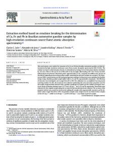
The most important metric of backbone networks is the available compression ratio, which is related to the network scale. If the size of the isolated subnet in G’ is small enough, then the probability of the backbone member is small and the network G’ has collapsed after removing the backbone from G. Based on the model of BA and the Eppstein Power law simulated by computer, we build the experimental networks at different scales to study the effective compression ratio. It is observed that the compression ratio changes of lar subgs size(G’) are shown in Figure 2. When the compression ratio compress ratio is large enough, then the size of maximum isolated subnet lar subgs size(G’) changes very little.

4. The Backbone Network Detect Algorithm The traditional backbone compression scheme is divided into the importance based on node and the shortest path. The former considers that the larger the degree, the more

where 𝛽 is a parameter and N(v) is the set of nodes connected to v. The definition of node importance based on the shortest path considers that the greater the number of nodes, the greater the importance of nodes. The definition of weight is shown in 󵄨󵄨 󵄨 󵄨{𝜋 ∈ Π (𝑥, 𝑦) : V ∈ 𝜋}󵄨󵄨󵄨 𝑤𝑝𝑎𝑡ℎ (V) ≡ ∑ 󵄨 (8) 󵄨 󵄨 |𝑉|2 󵄨󵄨󵄨Π (𝑥, 𝑦)󵄨󵄨󵄨 𝑥,𝑦∈𝑉 where Π(x, y) is the shortest path between node x and node y. 4.1. Extraction Process. In this paper, we propose an algorithm to extract backbone network with specific granularities according to user’s requirement, which is independent of network topology structure. The practical procedure includes two steps. In the first step, the initial hub node set H1 according to the topology potential of nodes is found. Secondly, the path is added based on the shortest path till the network is connective, and finally the backbone network is generated. A detailed description of these algorithm is given in Algorithm 1. 4.2. Discussion of the Algorithm Complexity. The shortest paths between all nodes in the network are calculated by using the breadth first search method. The time complexity is O(|𝑉||𝐸|) for undirected networks. The time complexity of calculating the topology potential of each node is O(|𝑉||𝐸|). Search backbone connections until the network is connective. The average shortest path length of the network is avg(Sp). The original subnet number of source is 𝛼|𝑉|. To make the original subnets connected, the backbone network is a tree structure, which means we need at least search O(𝛼|𝑉| ∗ |𝑉|avg(Sp)) links to make the network connective. So the complexity of the algorithm is O (max{𝛼|𝑉|2 𝑎V𝑔(𝑆𝑝), |𝑉||𝐸|}).

5. Evaluation To assess the efficiency of our backbone extraction approaches, we choose the public available datasets as the experiment dataset. We introduce the datasets briefly. Internet autonomy system networks (AS) are a collection of routers and links mapped from all ten ISPs with the biggest networks: AT&T, Sprint, and Verio, etc. These real networks are publicly available from [14]. All the data networks have nodes with scale from 600 to 900 and edges

Complexity

5

Input: network G, 𝛼(0 ≤ 𝛼 ≤ 1) Output: backbone B(𝛼) Matrix Sp: compute the shortest path length of all pairs of nodes; var i: = 1; Evaluate hops: = avg(Sp); evaluate factor: =√2/3∗avg(Sp); Begin: repeat: i: = i + 1; for each node v ∈G, compute 𝜑𝑖 (V):topology potential within i hops; sort(𝜑𝑖 (V), V ∈ 𝐺); source: =0; for each node v ∈G, if 𝜑𝑖 (V), V ∈ 𝐺 rank Top 𝛼, source:= source ∪{V}; repeat: for each pair of island subnets subg1,subg2∈source, if distance between subg1 and subg2 is the shortest, if distance(subg1, subg2) = 1 merge(subg1, subg2); else find neig1 ∈ subg1, 𝜑𝑖 (neig1) = max{𝜑𝑖 (v ∈ subg1)}, tie1 link neig1 and subg1 neig2 ∈ subg2, 𝜑𝑖 (neig2) = max{𝜑𝑖 (v ∈ subg2)}, tie2 link neig2 and subg2 source:= source ∪ {𝑛𝑒𝑖𝑔1, 𝑛𝑒𝑖𝑔2, 𝑡𝑖𝑒1, 𝑡𝑖𝑒2}; end if end if until network generated from source is connected B(𝛼) fl B(𝛼) ∪ source; until i ≥ hops End Algorithm 1: Detecting the backbone network based on topology potential.

5.1. Compression Ratio. In this paper we take the networks named as3356, as4755, as2914, and as7018 randomly and the numbers of nodes are 1786, 226, 11745, and 6253, respectively. In order to obtain the relevant parameters of backbone networks at different granularity, the number of isolated subnets cut subgs(G’) obtained by the backbone network under different selection ratios is evenly calculated. For instance, the scale control parameter starts from 0.01 to 1 and the step is set to 0.01. After the backbone network is generated, the compression ratio with the corresponding granularity can be obtained. Figure 3 shows the number of isolated subnets generated by each network with different compression ratios. Each pair of compression ratio and cut subgs(G’) corresponds to a point on the coordinate system, and the curves are fitted to these points. It is depicted that fitted curve is monotonically decreasing after increasing at the beginning, as illustrated in Figure 3. When the compression ratio increases to a certain value, the number of generated isolated subnets no longer changes. That is to say, it is no longer effective to compress the network

original network: as networks , the number of sub graphs while removing backbone from the original graph within different compression ratio

10000 9000 8000 number of sub graphs

with scale from 4000 to 10000. Each of them has about 400 backbone routers. High-energy physics theory citation network (hep-th) is collected from the e-print arXiv and covers all the citations within a dataset of 27,770 papers with 352,807 edges [15]. If paper i cites paper j, a directed edge is connected from i to j. If a paper cites or is cited by a paper outside the dataset, then the graph does not contain any information about this.

7000 6000 5000 4000 3000 2000 1000 0

0

0.1 0.2 0.3 0.4 0.5 0.6 0.7 0.8 0.9 compression ratio as7018, invalid as7018, effective as3356, invalid as3356, effective

1

as4755, invalid as4755, effective as2914, invalid as2914, effective

Figure 3: The number of generated isolated subnets with different compression ratio.

continuously to reduce the connectivity of the network. The solid line in the fitting curve denotes effective compression, and the dashed part denotes invalid compression. Measuring the performance of backbones networks needs to exclude the situation of invalid compression ratio. In the Internet

6

Complexity Table 1: Comparison with the precision ratio and recall ratio [13]. as1239

CM

PR 0.91 0.94 0.95 0.77

Deg/All Beta/All Path/all TP method

PR 0.97 0.89 1.00 0.76

as7018 as3356 as4755 as2914

0.9 0.8 0.7 0.6 0.5 0.4 0.3 0.2 0.1 0

0

0.1

0.2

0.3

0.4 0.5 0.6 0.7 Compression ratio

0.8

0.9

1

Compression Ratio

0.2 0.15 0.1 0.05 0

as4755

as3356

as2914

as7018

as1239

1 0.9 0.8 0.7 0.6 0.5 0.4 0.3 0.2 0.1 0

Precision Ratio, Recall Ratio

Figure 4: The optimal compression ratios of different networks. 0.25

as3356 RR 0.19 0.27 0.14 0.28

Test-bed: as- networks

1 Max size of the generated fragments of ＇

as2914 RR 0.27 0.35 0.17 0.47

Precision Ratio Recall Ratio Compression Ratio

Figure 5: The optimal parameters of the extracted Internet mapping network.

mapping results, the optimal compression ratios of the networks as3356, as4755, as2914, and as7018 are about 0.23, 0.16, 0.08, and 0.035, respectively, as illustrated in Figure 4. 5.2. Precision Ratio and Recall Ratio. Measuring the performance of backbone network is to explore the optimal highperformance network metrics. For a large-scale network, it is impossible to calculate the backbone at the whole granularities, as the time complexity will be quite high. Using the binary optimization strategy, when the dichotomous range is small enough, we can determine the maximum effective

PR 0.93 0.97 0.97 0.86

as7018 RR 0.18 0.22 0.16 0.73

PR 0.91 0.91 0.96 0.61

RR 0.21 0.24 0.11 0.58

compression ratio. For example, if the range is set to 0.01, the search time is log1/2 (0.01) ∼ 7. After discovering the maximum effective compression ratio, we search the optimal compression ratio and the corresponding optimal backbone network. The Internet mapping network has real backbone node data; thus we can compare the extracted backbone network to verify the extraction results on the real backbone network. The optimal parameters to evaluate the extracted backbone are shown in Figure 5. Compared with the traditional methods adopted in [7], it is found that these methods can obtain high precision ratios about the value of 0.9, while the recall ratios of the traditional methods are lower than 0.2. On the other hand, the precision ratio of the topology potential extraction method (named TP method) is approximately 0.8 and the recall ratio increased to about 0.5. Since an excellent extraction method requires a higher recall ratio, our method is superior to the traditional methods from this aspect. Other related extraction algorithms do not have real instance verification, and the extraction quality is unknown and lacks verification. Part of the experimental results is listed in Table 1. The abbreviation of compressing method is CM, precision ratio is PR, and the recall ratio is RR. 5.3. Coverage of Backbone with Various Hops. Taking the Hep-th network as experimental data, we analyze the coverage performance of backbone networks with different hops. In this paper, the range of hops is adopted from 2 to 7. Firstly, we take the traditional centrality measurement, degree, betweenness, and closeness to analyze, as shown in Figure 6. We compute the node important properties of the generated backbone network with various hops. The coordinate point indicates the nodes proportions of the backbone network sorted the top i to the nodes of the original network sorted the top ranki , defined as coverage(i). The important attributes are node degree (the upper left), node betweenness (the upper right), node closeness (the lower left), and edge betweenness (the lower right). The results show that using different centrality metrics to measure the extraction results with various hops has different advantages. For example, when the metric is degree, using 2 hops can get the best extraction effect. When the metric is closeness, using 7 hops can get the best extraction effect. Therefore, in this paper, we use the topology potential to extract backbone networks with specific granularities according to user’s requirement, which is independent of network topology structure. We can get the comprehensive results of extracted backbone network.

Complexity

7 node degree

1

hops value is 2 hops value is 3 hops value is 4 hops value is 5 hops value is 6 hops value is 7 Ex(coverage)

0.8

0.6

0.7

0.5 0.4

0.6 0.5 0.4

0.3

0.3

0.2

0.2

0.1

0.1 0

100

200

300 i

400

500

0

600

node closeness

1

0.8 0.7 0.6

0

100

200

0.35

hops value is 2 hops value is 3 hops value is 4 hops value is 5 hops value is 6 hops value is 7 Ex(coverage)

0.9

coverage(i)

0.8

300 400 i edge betweenness

0.25

0.5 0.4 0.3

500

600

hops value is 2 hops value is 3 hops value is 4 hops value is 5 hops value is 6 hops value is 7 Ex(coverage)

0.3

coverage(ei )

coverage(i)

0.7

hops value is 2 hops value is 3 hops value is 4 hops value is 5 hops value is 6 hops value is 7 Ex(coverage)

0.9

coverage(i)

0.9

0

node betweenness

1

0.2 0.15 0.1

0.2 0.05

0.1 0

0

100

200

300 i

400

500

600

0 0

100

200

300

ei

400

500

600

Figure 6: The coverage of backbone in various hops.

6. Conclusion

Acknowledgments

In this paper, we introduced the topology potential to solve the problem of backbone network extraction. Based on the novel topology measurement, an algorithm is proposed to extract backbone networks at different granularities. In order to detect the optimal backbone extraction granularity, an evaluation metric that considers the tradeoff between network connectivity and network properties is presented. By experiments on the public available datasets of Internet AS network and the Hep-th Network, it is proven that the precision ratio and recall ratio to extract the backbone network are superior to current methods. In the future, we will investigate the performance of backbone network at different scale and the dynamic evolution properties.

This work was supported by National Key Research and Development Plan of China (2016YFB0502600, 2016YFC0803000), National Natural Science Fund of China (61472039), International Scientific and Technological Cooperation and Academic Exchange Program of Beijing Institute of Technology (GZ2016085103), and Frontier and Interdisciplinary Innovation Program of Beijing Institute of Technology (2016CX11006).

Conflicts of Interest There is no conflict of interests related to this paper.

References [1] R. K. Darst, C. Granell, A. Arenas, S. G´omez, J. Saram¨aki, and S. Fortunato, “Detection of timescales in evolving complex systems,” Scientific Reports, vol. 6, 2016. [2] A. Holzinger and I. Jurisica, “Knowledge discovery and data mining in biomedical informatics: The future is in integrative, interactive machine learning solutions,” in Interactive knowledge discovery and data mining in biomedical informatics, pp. 1–18, Springer, Berlin, Germany, 2014.

8 [3] A. Y. Wu, M. Garland, and J. Han, “Mining scale-free networks using geodesic clustering,” in Proceedings of the tenth ACM SIGKDD international conference on Knowledge discovery and data mining, pp. 719–724, August 2004. [4] S. Scellato, A. Cardillo, V. Latora, and S. Porta, “The backbone of a city,” The European Physical Journal B, vol. 50, no. 1-2, pp. 221–225, 2006. [5] C. E. Hutchins and M. Benham-Hutchins, “Hiding in plain sight: criminal network analysis,” Computational and Mathematical Organization Theory, vol. 16, no. 1, pp. 89–111, 2010. [6] J. H. Choi, G. A. Barnett, and B.-S. Chon, “Comparing world city networks: a network analysis of Internet backbone and air transport intercity linkages,” Global Networks, vol. 6, no. 1, pp. 81–99, 2006. [7] D. Nan, W. Bin, and W. Bai, “A Parallel Algorithm for enumerating all Maximal Cliques in Complex Networks,” in Proceedings of the The 6th ICDM 2006 Mining Complex Data Workshop, IEEE Computer Society, pp. 320–324, New Orleans, LA, USA, 2006. [8] C. Gilbert and K. Levchenko, “Compressing Network Graphs[C],” in Proceedings of the Link KDD Workshop at the 10th ACM Conference on KDD, 2004. [9] W. Yao, Y. Yang, and G. Tan, “Recursive Kernighan-Lin algorithm (RKL) scheme for cooperative road-side units in Vehicular networks,” Communications in Computer and Information Science, vol. 405, pp. 321–331, 2014. [10] S. A. Stoev, G. Michailidis, and J. Vaughan, “On global modeling of backbone network traffic,” in Proceedings of the 29th Conference on Computer Communications (INFOCOM ’10), pp. 1–5, San Diego, CA, USA, March 2010. [11] Liqiang Qian, Zhan Bu, Mei Lu, Jie Cao, and Zhiang Wu, “Extracting Backbones from Weighted Complex Networks with Incomplete Information,” Abstract and Applied Analysis, vol. 2015, Article ID 105385, 11 pages, 2015. [12] H. Yanni, H. Jun, L. Deyi, and Z. Shuqing, “A novel measurement of structure properties in complex networks,” in Proceedings of the International Conference on Complex Sciences, pp. 1292–1297, 2009. [13] N. He, W. Gan, and D. Li, “Evaluate Nodes Importance in the Network Using Data Field Theory,” in Proceedings of the 2007 International Conference on Convergence Information Technology (ICCIT 2007), pp. 1225–1234, November 2007. [14] N. Spring, R. Mahajan, and D. Wetherall, “Measuring ISP topologies with Rocketfuel,” ACM SIGCOMM Computer Communication Review, vol. 32, no. 4, pp. 133–145, 2002. [15] “SNAP network datasets,” https://snap.stanford.edu/data/ cit-HepTh.html.

Complexity

Advances in

Operations Research Hindawi www.hindawi.com

Volume 2018

Advances in

Decision Sciences Hindawi www.hindawi.com

Volume 2018

Journal of

Applied Mathematics Hindawi www.hindawi.com

Volume 2018

The Scientific World Journal Hindawi Publishing Corporation http://www.hindawi.com www.hindawi.com

Volume 2018 2013

Journal of

Probability and Statistics Hindawi www.hindawi.com

Volume 2018

International Journal of Mathematics and Mathematical Sciences

Journal of

Optimization Hindawi www.hindawi.com

Hindawi www.hindawi.com

Volume 2018

Volume 2018

Submit your manuscripts at www.hindawi.com International Journal of

Engineering Mathematics Hindawi www.hindawi.com

International Journal of

Analysis

Journal of

Complex Analysis Hindawi www.hindawi.com

Volume 2018

International Journal of

Stochastic Analysis Hindawi www.hindawi.com

Hindawi www.hindawi.com

Volume 2018

Volume 2018

Advances in

Numerical Analysis Hindawi www.hindawi.com

Volume 2018

Journal of

Hindawi www.hindawi.com

Volume 2018

Journal of

Mathematics Hindawi www.hindawi.com

Mathematical Problems in Engineering

Function Spaces Volume 2018

Hindawi www.hindawi.com

Volume 2018

International Journal of

Differential Equations Hindawi www.hindawi.com

Volume 2018

Abstract and Applied Analysis Hindawi www.hindawi.com

Volume 2018

Discrete Dynamics in Nature and Society Hindawi www.hindawi.com

Volume 2018

Advances in

Mathematical Physics Volume 2018

Hindawi www.hindawi.com

Volume 2018