Proceedings of the XIVth International Symposium on High Voltage Engineering, Tsinghua University, Beijing, China, August 25-29, 2005
G-005
A New Procedure for Partial Discharge Localization in Gas-Insulated Switchgears in Frequency Domain Stefan M. Hoek1*, Uwe Riechert2, Thomas Strehl3, Stefan Tenbohlen1 and Kurt Feser1 1 University of Stuttgart, IEH, Pfaffenwaldring 47, 70569 Stuttgart, Germany 2 ABB Switzerland Ltd - Gas Insulated Switch Systems, Zürich, Switzerland 3 LEMKE DIAGNOSTICS GmbH in Volkersdorf / Dresden, Germany * E-Mail:
[email protected] locating is the measurement with the time-of-flight method. By the time-of-flight technique the time difference between the wave fronts arriving at two UHF- PD - sensor indicate the location of the PD source. The time difference (∆t) is usually in tens of 1 ns, so that a fast digital acquisition has to be applied for measurements [3].
Abstract: This new method will permit a cost-efficient localisation of partial discharges (PD) in gas-insulated switchgears (GIS). It uses the interference phenomenon of two superimposed sensor signals. The signal interference results in the time delay (∆t) between the two signals. Evaluating this time delay a localization is possible. Two related sensor signals are required to receive acceptable results for the measurement procedure. Considering the dispersion effects of higher modes in GIS only a certain frequency range is useful for the measurement. The interferences can be measured at various setups. INTRODUCTION The liberalization of the energy market forces utilities to reduce costs. A condition based, effective and fast maintenance strategy is essential. Considering the maintenance strategy of GIS, a sensitive PD detection is essential to detect defects. The type of the PD defect can be recognized with different proved methods like pattern recognition with the phased resolved partial discharge (PRPD) analyses or other techniques. To assess the risk of a defect, its location is additionally important. Thus, a sensitive PD detection with estimation of the nature of the defect and a fast and exact locating is advantageous. Hence the demand for reliable and economic measurement tools to locate PDsources is still increasing.
Fig. 1: Cross section of a GIS The distance X1 can be calculated with the equation (1) in case the time difference (∆t) is known. X represents the distance between the sensors and c0 is the propagation speed of the wave in the GIS (c0 = 0.3 m/ns) [3].
X1 =
PD LOCATING IN GIS
X − ( X 2 − X 1 ) X − c0 ⋅ ∆t = 2 2
(1)
The time difference is determined by the initial impulse steepness of the two signals. If the initial start of the signal is not totally clear or there are different signal-tonoise ratios (SNR) of the two signals, the measurement of the time difference ∆t is not easy detectable in all cases.
Several methods can be used, based on different physical phenomena. Methods based on a time delay evaluation between different propagating modes [1] and directional couplers [2], have shown to be unpractical [3]. The most practical methods are based on sectionizing, electrical time-of-flight measurements, acoustic measurement and a combination of all of them. Another newly investigated method, presented in this paper, uses the interference measurement in the frequency domain. Measurements in frequency domain features various advantages like less hardware effort compared to conventional methods in time domain.
Interference measurement
Another method to localize PD in GIS is to use the frequency domain. The interference phenomena of two sensor signals, which are added, should give information about the time delay (∆t) between the signals. A measurement procedure with a spectrum analyser instead of a cost-intensive fast digital oscilloscope, would be more economical.
Locating in time domain Very fast electric pulses with rise times below 1 ns, emitted by a PD source, propagate in all directions along the GIS duct. A simple and obvious way of
The idea is based on the displacement law of a FourierTransformation of the received signals.
1
Proceedings of the XIVth International Symposium on High Voltage Engineering, Tsinghua University, Beijing, China, August 25-29, 2005
[
FFT f (t − ∆t
)] = FFT [ f (t )]⋅ e
− jω∆t
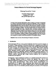
propagate at frequencies above their own critical frequency (fc). TEM-modes have no critical frequency and will propagate starting from 0 Hz. The critical frequencies depends on the geometry of the GIS. With an increasing cross section of the GIS, the critical frequency is decreasing. In Fig. 3 the critical frequencies of the first wave modes are shown for three different types of GIS [5].
(2)
Measurement procedure To visualise the interference phenomena it is insufficient to make only one measurement. There are three power spectrums needed, which are compared in a characteristic way. The power spectrum is the absolute value of the complex FFT. The three power spectrums are obtained from Sensor 1 (3), Sensor 2 (4) and the added signal of Sensor 1 and 2 (5) with a conventional spectrum analyser. The last signal is obtained with a RF power splitter, with no further reflections or other disturbing influences (Fig. 10).
1800
Critical frequency (MHz)
F (ω ) = FFT [ f (t )]
(3)
G (ω ) = FFT [g (t )]
(4)
H (ω ) = FFT [g (t ) + f (t − ∆t )]
G-005
1600
550 kV
1400
362 kV
1200
300 kV
These three resulting signals are combined in (6). So the time difference (∆t) will be estimable with the resulting cosine function in case of f(t) = g(t).
717
600 521 267
TEM
TE11
TE21
TE31
TM02
TE02 / TM11
fc f
(7)
Below the lowest critical frequency of all modes (in GIS the fc of TE11), only TEM-modes are able to propagate. In this frequency range less dispersion effects exists and the interferences can be recognized. To measure in the frequency range below the first critical frequency, a low pass filter is applied, because the signal energy in the higher modes is much higher than in the TEM-mode (Fig. 10). One Requirement for a successful measurement is a sensitive measurement in this frequency range. All other effects influencing the signal within the GIS should be eliminated.
ω ⋅ ∆t cos 2
-30 1300 1350 Frequency [MHz]
851
The group velocity (vg) of the TE- / TM-wave modes is frequency dependent which is a precondition for dispersion. The speed of the higher wave modes can be calculated according to the following equation [6].
(6)
-10
1250
805
Fig. 3: Critical frequencies (fc) within an GIS for 300 kV, 362 kV and 550 kV
0
1200
721
508
377
v g ( f ) = c0 ⋅ 1 −
-20
1196
1016
Wave modes
This cosine function has equidistant minima (see Fig. 2) which can be interpreted as interference phenomena [4].
[dB]
991
800
0
H (ω ) ω ⋅ ∆t = cos F (ω ) + G (ω ) 2
1133
400
1651
1404
1000
200
(5)
1564
1400
Fig. 2: Resulting cosine function from (6) for a ∆t = 40 ns Requirements Two related signals are required to obtain useful results from equation (6). Unfortunately this represents not a normal case in GIS. Current studies show that an magnitude difference is not critical if the nature of both signals is similar. For different magnitudes, the combined function (6) changes to the absolute value of a cosine function with decreased magnitude and an offset. To keep the characteristics of both signals similar the effect of dispersion should be kept as small as possible.
Measurement example The following measurement shows the method with a simplified setup. A pulse generator excites the signal in two cables with different length to generate the time difference (∆t). An attenuator reduces the magnitude of one signal. For a better understanding the time-domain measurement is also visualized. They are in general not necessary for the procedure.
Three different types of wave modes which propagate in the GIS are distinguished. The TMmn-mode (Hz = 0), the TEmn-mode (Ez = 0) and the TEM-mode (Hz = 0, Ez = 0) (m and n mark the different types of wave modes). Every wave mode, except the TEM-mode, has its own critical frequency (fc). Higher modes are able to
2
Proceedings of the XIVth International Symposium on High Voltage Engineering, Tsinghua University, Beijing, China, August 25-29, 2005
G-005
B
0
B
Amplitude [V]
Amplitude [V]
0 -1
f (t )
-2 -3 -5 0
-1
g (t ) + f (t − ∆t )
-2 -3
0
50
100 150 T im e [n s ]
200
-5 0
250
0
50
100 150 T im e [n s ]
200
-20
-50
250
A
FFT [ f (t )] -30 Amplitude [dBm]
Amplitude [dBm]
-55
-60
-65
-50
-60
-70 200
-40
400
600
800 1000 Frequency [MHz]
1200
1400
-70 200
Fig. 4: Time domain measurement f(t) and power spectrum F(ω)
FFT [g (t ) + f (t − ∆t )] 400
600
800 1000 Frequency [MHz]
1200
1400
Fig. 6: Time domain measurement and power spectrum H(ω) of both signals (summed with the power splitter).
B
4
Amplitude [V]
0 -1
g (t )
2
-2
0
-5 0
0
50
100 150 T im e [n s ]
200
[dB]
-3 250
-2 -4
FFT [g (t )] + FFT [ f (t )]
-6
-35 Amplitude [dBm]
FFT [g (t ) + f (t − ∆t )]
A
-30
-40
-8 200
-45
400
600
800 1000 Frequency [MHz]
1200
1400
-50
Fig. 7: The calculated combination of the power spectra
-55 -60
FFT [g (t )]
-65 -70 200
400
600
800 1000 Frequency [MHz]
1200
1
1400
theoretical cosine
0
Fig. 5: Time domain measurement g(t) and power spectrum G(ω)
[dB]
-1
The time difference is measured in the time domain (Fig. 4 and Fig. 5) as ∆t = 39,3 ns. These three power spectrums (Fig. 4, Fig. 5 and Fig. 6) are combined in the way presented in equation (6) using a software (Fig. 7).
-2 -3 -4 -5 1200
1250
1300 Frequency [MHz]
1350
1400
Fig. 8: Magnification of the power spectra (Fig. 7) with the theoretical cosine (6)
3
Proceedings of the XIVth International Symposium on High Voltage Engineering, Tsinghua University, Beijing, China, August 25-29, 2005
The signal in Fig. 8 shows an interference phenomenon and has equidistant minima. There are minima for example at 1210 MHz, 1235 MHz, and at 1260 MHz and further on. The characteristic frequency ∆f equals 25 MHz and with the following equation
∆t =
C
20
theoretical cosine
G
15 10 [dB]
1 ∆f
G-005
(8)
5 0 -5 -10
the estimated time difference (∆t) is 1/∆f = 40 ns.
-15 50
The relation to the theoretical cosine shows that this interference phenomenon is useful although the signal f(t) is not exactly the same as g(t) caused by a attenuator.
150 200 Frequency [MHz]
250
300
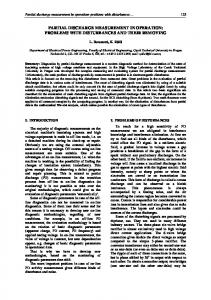
Fig. 11: Calculated combination of the power spectra of the measurement at the 550 kV GIS The time difference is estimable in time domain measurements as ∆t = 95.6 ns. The combined signal in Fig. 11 shows interference phenomena. The best matching with the theoretical cosine function is at ∆f = 10.54 MHz and in respect of equation (8) ∆t can be calculated as ∆t = 94.9 ns. The interference phenomena in the calculated combination of the power spectra (Fig. 11) are clearly visible. At other GIS types and test setups these interferences are also recognizable (Fig. 13, Fig. 14).
Measurement at a real GIS The same interference effect can also be measured in an existing GIS. In the following different test setups with different types of GIS and PD-sources the interferences are presented as in Fig. 11. Locating of a PD-source is possible in a 9 m long GIS (Fig. 9) for 550 kV in our lab with or without termination with wave impedance. The sensors are conventional UHF-PD-sensors. The connection cable to the sensors are different in length to increase the absolute ∆t (Fig. 10). The PD-source is a pulse generator with an antenna (with a equivalent magnitude according to IEC 60270 q = approx. 50 pC).
The measurement of interference phenomena in a 3 m long GIS of 362 kV nominal voltage (Fig. 12) with conventional UHF-PD-Sensors and a protrusion on the outer conductor as PD-source (according to IEC 60270 q = approx. 150 pC) is shown in Fig. 13.
UHF-PD-sensor
termination
100
PD-source
PD-source
Fig. 9: 550 kV GIS with a PD-source and UHFSensors UHF-sensor spectrum analyser
RF power splitter
325 kV test transformer
f(t-∆t)+g(t) f(t-∆t)
g(t) amplif ier
low pass connection cable with diff. length
Sensor 1
Fig. 12: GIS (362 kV) with PD-source The best matching of the calculated combination with the theoretical cosine function (Fig. 13) is at ∆f = 14.1 MHz and with equation (8) ∆t is 70.7 ns (time domain measurements shows ∆t = 73.5 ns).
Sensor 2 el. PD-Impuls
Fig. 10: Cross section of a GIS with corresponding test setup
4
Proceedings of the XIVth International Symposium on High Voltage Engineering, Tsinghua University, Beijing, China, August 25-29, 2005
-10
Two similar sensor signals are required to receive useable results from this measurement procedure. Only the TEM-mode is useful for the measurement, because of dispersion effects at higher modes. These interferences can be measured at all different arrangements. However, the correct interpretation of these signals is in some cases a complex procedure, and requires sophisticated knowledge.
-15
REFERENCES
theoretical cosine 5 0 [dB]
G-005
-5
100
150
200 Frequency [MHz]
250
[1] M. C. Zhang, H. Li, TEM- and TE-Mode Waves Excited by Partial Discharges in GIS, ISH London, 22.-27. August 1999, pp 5.144.P5-5.147.P5
300
Fig. 13: The calculated combination of the power spectra of the measurement at the 362 kV GIS
[2] G. Schöffner, A Directional Coupler System for the Direction Sensitive Measurement of UH-PD Signals in GIS and GIL, CEIDP 2000, pp 634-638.
The measurement of the interference phenomena in a complete bay of a 300 kV GIS is shown in Fig. 14. The two sensors are conventional UHF-PD-sensors at the bus bar and at the termination of the GIS. This distance corresponds to the distance of sensors at installed GIS. The PD-source is a pulse generator with an antenna.
[3] CIGRE TF 15/33.03.05, PD Detection System for GIS: Sensitivity Verification for the Method and the Acoustic Method, Electra No 183, April 1999 [4] S. M. Hoek, K. Feser, Partial discharge (PD) locating in gas-insulated switchgears (GIS), 12th Workshop on High Voltage Engineering, Lübbenau / Spreewald, Germany, 20.-24. September 2004, Book of Abstracts, pp. 2-3
5
0
[5] R. Kurrer, K. Feser, The Application of Ultra-HighFrequency Partial Discharge Measurements to Gas-Insulated Substations, IEEE Transactions on Power Delivery, Vol. 13, No. 3, July 1998
[dB]
-5
-10
[6] Meinke, Grundlach, Taschenbuch der Hochfrequenztechnik, 4. Aufl., Springer-Verlag, 1985
-15
theoretical cosine 100
150
200 250 Frequency [MHz]
300
350
Fig. 14: Calculated combination of the power spectra of the measurement at the 300 kV GIS The theoretical cosine function matches best at ∆f = 21.2 MHz so ∆t is measured as 47 ns (time domain measurement ∆t = 45 ns). Because of the more complex arrangement the evaluation of the measurement at 362 kV and 300 kV GIS (Fig. 13, Fig. 14) is not as simple as the measurement at the 550 kV GIS. The additional reflections of this arrangement in the GIS itself is the reason. The interpretation of these signals measured in a complex GIS will be the topic of future research work. RESULTS AND DISCUSSION
This new method allows a cost-effective localization of PD in GIS in at least basic configurations or in gasinsulated lines (GIL). The interference phenomena of two sensor signals, which are summed, results in information about the time delay (∆t) between the signals. With this information a localization is possible.
5