Design Issues in a Multiobjective Cellular Genetic Algorithm - CiteSeerX

Design Issues in a Multiobjective Cellular Genetic Algorithm Antonio J. Nebro, Juan J. Durillo, Francisco Luna, Bernab´e Dorronsoro, Enrique Alba ? Departamento de Lenguajes y Ciencias de la Computaci´ on E.T.S. Ingenier´ıa Inform´ atica Campus de Teatinos, 29071 M´ alaga (Spain) antonio,durillo,flv,bernable,[email protected]

Abstract. In this paper we study a number of issues related to the design of a cellular genetic algorithm (cGA) for multiobjective optimization. We take as an starting point an algorithm following the canonical cGA model, i.e., each individual interacts with those ones belonging to its neighborhood, so that a new individual is obtained using the typical selection, crossover, and mutation operators within this neighborhood. An external archive is used to store the non-dominated solutions found during the evolution process. With this basic model in mind, there are many different design issues that can be faced. Among them, we focus here on the synchronous/asynchronous feature of the cGA, the feedback of the search experience contained in the archive into the algorithm, and two different replacement strategies. We evaluate the resulting algorithms using a benchmark of problems and compare the best of them against two state-of-the-art genetic algorithms for multiobjective optimization. The obtained results indicate that the cGA model is a promising approach to solve this kind of problem.

1

Introduction

Most optimization problems in the real world are multiobjective in nature. This feature, along with the facts that function evaluations can require a significant computation time and the search spaces tends to be very large, make metaheuristics popular techniques to solve multiobjective optimization problems (MOPs). Among them, evolutionary algorithms have been investigated by many authors, and some of the most well-known algorithms for solving MOPs belong to this class (e.g. NSGA-II [1], PAES [2], SPEA2 [3]). Nevertheless, in recent years there is a trend to adapt other kinds of metaheuristics (sometimes called “alternative methods”, with reference to evolutionary algorithms) to the multiobjective field, such as tabu search [4] or scatter search [5]. ?

This work has been partially funded by the Ministry of Science and Technology and FEDER under contract TIN2005-08818-C04-01 (the OPLINK project).

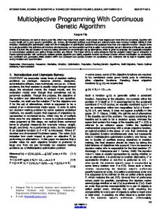
(a)

(b)

(c)

Fig. 1. Panmictic (a), distributed (b), and cellular (c) GAs

Many evolutionary algorithms for solving MOPs are some kind of genetic algorithm (GA). These algorithms work over a set (population) of potential solutions (individuals) which undergoes stochastic operators in order to search for better solutions. These operators are typically selection, crossover, and mutation. Most GAs use a single population (panmixia) of individuals and apply the operators to them as a whole (see Fig. 1a). Conversely, there exist the so-called structured GAs, in which the population is decentralized somehow. Among the many types of structured GAs, the distributed and cellular models are two popular variants [6, 7] (see Fig. 1b and Fig. 1c, respectively). In many cases, these decentralized algorithms provide a better sampling of the search space, resulting in an improved numerical behavior with respect to an equivalent algorithm in panmixia. In this work, we focus on the cellular model of GAs (cGAs). This kind of GAs uses the concept of (small) neighborhood in the sense that an individual may only interact with its nearby neighbors in the breeding loop [8–10]. The overlapped small neighborhoods of cGAs help in exploring the search space because the induced slow diffusion of solutions through the population provides a kind of exploration (diversification), while exploitation (intensification) takes place inside each neighborhood by genetic operations. It is worth mentioning that the neighborhood is defined among tentative solutions in the algorithm, with no relation to the geographical neighborhood definition in the problem space. cGAs have proven to be very effective tools for solving a diverse set of single objective optimization problems from both classical and real world settings [11, 12], but little attention has been paid to their use in the multiobjective optimization field [13–17]. In [18] we proposed the MultiObjective Cellular (MOCell) algorithm, which, together with cMOGA [16] is the unique existing adaptation of the canonical cGA model to the multiobjective field. MOCell uses an external archive to store the non-dominated solutions found during the execution of the algorithm, like many other multiobjective evolutionary algorithms do (e.g., PAES, SPEA2). MOCell is characterized by selecting a fixed number of individuals from the archive to replace the same number of randomly chosen individuals from the population (archive feedback) at the end of each iteration of the algorithm. This is carried out with the hope of taking advantage of the search experience in order to find a Pareto front with good convergence and spread. This new

replacement coexists with the typical replacement of a canonical cGA, in which the newly generated individual replaces the current one if the latter is worse than the former. However, there are many other different strategies that could be applied in the context of MOCell. In this paper we explore three possibilities. Firstly, MOCell is a synchronous cGA, in the sense that the cell updates are carried out simultaneously; we consider here the alternative of implementing an asynchronous approach, in which the cell updates are performed in a sequential order [12]. Secondly, we study an alternative way to explicit feedbacking which lies in the selection of an individual from the archive to be matched to the one taken from the neighborhood in the reproductive cycle. Thirdly, in the context of an asynchronous cGA, instead of considering the current individual to be replaced, it is possible to consider all the neighborhood, i.e., the new individual replaces the worst one in the neighborhood. The contributions of our work can be summarized as follows: – We explore three different design issues in the MOCell algorithm to study their influences in the accuracy of the algorithm. – The resulting configurations are validated using two benchmarks: the ZDT family of MOPs [19], which is used in many studies in the field, and a benchmark constructed using the WFG Toolkit [20]. – The experiments are carried out using a rigorous statistical analysis around three performance metrics. – In order to determine how competitive the resulting algorithm is, we compare the MOCell version yielding the best results against NSGA-II and SPEA2. The remaining of the paper is organized as follows. In Section 2, we discuss related works concerning cGAs and multiobjective optimization. In Section 3, we describe MOCell and propose six variants of it, resulting from combining three different features. Experimental results are presented in Section 4. Finally, in Section 5 we give some conclusions and lines for future research.

2

Related Work

In this section we discuss related works about cGAs and multiobjective optimization. As mentioned in the introduction, only few works can be found in the literature. In [13, 17], two multiobjective evolution strategies following a predator-prey model are presented. This is a model similar to a cGA, because solutions (preys) are placed on the vertices of an undirected connected graph, thus defining neighborhoods, where they are ‘caught’ by predators. Murata and Gen presented in [14] an algorithm in which, for an n-objective MOP, the population is structured in an n-dimensional weight space, and the location of individuals (called cells) depends on their weight vector. Thus, the information given by the weight vector of individuals is used for guiding the search. Notice that in this work the neighborhoods are defined in the objective

space, instead of in the location of individuals in the topology of the population, as it is in classical cGAs. A metapopulation evolutionary algorithm (called MEA) is presented in [15]. This algorithm follows a cellular model with the peculiarity that disasters can occasionally happen in the population, thus killing all the individuals located in the disaster areas (extinction). Additionally, these empty areas produced by disasters can also be occupied by individuals (colonization). Thus, this model allows a flexible population size, combining the ideas of cellular and spatially distributed populations. Alba et al. proposed in [16] cMOGA, a cellular multiobjective algorithm which, in contrast to the aforementioned works, is based on the canonical cGA model. This algorithm uses an external archive to store the non-dominated solutions found during the search. This feature was included in MOCell [18], which can be considered as an evolution of cMOGA in which a feedback from the archive to the population has been included. MOCell was compared in [18] to the algorithms NSGA-II and SPEA2 using a benchmark of both unconstrained and constrained bi-objective MOPs, obtaining competitive results in convergence and clearly outperforming the other algorithms in terms of diversity.

3

The Algorithm

In this section we first detail a description of a canonical cGA; then, we describe the algorithm MOCell and its different configurations that we intend to study. 3.1

Canonical cGA Model

A canonical cGA follows the pseudo-code included in Algorithm 1. In this basic cGA, the population is usually structured in a regular grid of d dimensions (d = 1, 2, 3), and a neighborhood is defined on it. The algorithm iteratively considers as current each individual in the grid (line 3). An individual may only interact with individuals belonging to its neighborhood (line 4), so its parents are chosen among its neighbors (line 5) with a given criterion. Crossover and mutation operators are applied to the individuals in lines 6 and 7, with probabilities Pc and Pm , respectively. Afterwards, the algorithm computes the fitness value of the new offspring individual (or individuals) (line 8), and inserts it (or one of them) into the equivalent place of the current individual in a new auxiliary population (line 9) following a given replacement policy. After each generation (or loop), the auxiliary population is assumed to be the population for the next generation. This loop is repeated until a termination condition is met (line 2). The most usual termination conditions are to reach the optimal value, to perform a maximum number of fitness function evaluations, or a combination of both of them. According to this canonical cGA, all the cells can be updated in parallel, yielding the so-named synchronous cGA. The alternative is the asynchronous cGA, in which the cells are updated one at a time in some sequential order. An

Algorithm 1 Pseudocode for a Canonical cGA 1: proc Steps Up(cga) //Algorithm parameters in ‘cga’ 2: while not Termination Condition() do 3: for individual ← 1 to cga.popSize do 4: n list←Get Neighborhood(cga,position(individual)); 5: parents←Selection(n list); 6: offspring←Recombination(cga.Pc,parents); 7: offspring←Mutation(cga.Pm,offspring); 8: Evaluate Fitness(offspring); 9: Replace(position(individual),offspring,cga,aux pop); 10: end for 11: cga.pop←aux pop; 12: end while 13: end proc Steps Up;

Algorithm 2 Pseudocode of MOCell 1: proc Steps Up(mocell) //Algorithm parameters in ‘mocell’ 2: Pareto front = Create Front() //Creates an empty Pareto front 3: while not TerminationCondition() do 4: for individual ← 1 to mocell.popSize do 5: n list←Get Neighborhood(mocell,position(individual)); 6: parents←Selection(n list); 7: offspring←Recombination(mocell.Pc,parents); 8: offspring←Mutation(mocell.Pm,offspring); 9: Evaluate Fitness(offspring); 10: Replacement(position(individual),offspring,mocell,aux pop); 11: Insert Pareto Front(offspring); 12: end for 13: mocell.pop←aux pop; 14: mocell.pop←Feedback(mocell,ParetoFront); 15: end while 16: end proc Steps Up;

asynchronous cGA can be easily obtained from Algorithm 1 assuming that the cells are sequentially updated, so the auxiliary population is not needed in the algorithm. 3.2

A Multiobjective cGA: MOCell

In this section we describe MOCell, a multiobjective metaheuristic based on the previously explained cGA model. Its pseudo-code is given in Algorithm 2. We can observe that Algorithms 1 and 2 are very similar. One of the main differences between the two algorithms is the existence of a Pareto front in the multiobjective case. The Pareto front is just an additional population (the external archive) composed of the non-dominated solutions found. The archive has a maximum size and, therefore, the insertion of solutions in the Pareto front has to be carefully managed to obtain a diverse set. Hence, a density estimator is needed to remove solutions from the archive when it becomes full. MOCell starts by creating an empty Pareto front (line 2 in Algorithm 2). Individuals are arranged in a 2-dimensional toroidal grid, and the genetic operators are successively applied to them (lines 7 and 8) until the termination condition is met (line 3). Hence, for each individual, the algorithm selects two parents from its neighborhood, recombines them in order to obtain an offspring,

mutates this offspring, and evaluates the resulting individual; then the algorithm decides whether the new offspring replaces the current one (line 10). The next step (line 11) is to insert the offspring into the external archive, if appropriate. Finally, after each generation, the old population is replaced by the auxiliary one (line 13), and a feedback procedure is invoked to replace a number of randomly chosen individuals by a number of solutions from the archive (line 14). In this algorithm, the resulting offspring replaces the individual at the current position if the former is better than the later, but, as it is usual in multiobjective optimization, we need to define the concept of “best individual”. Our approach is to replace the current individual if it is dominated by the offspring or both the two are non-dominated and the current individual has the worst crowding distance (as defined in NSGA-II) in a population composed of the neighborhood plus the offspring. This criterion is also used to decide whether the offspring solutions are added to the external archive (line 11 in Algorithm 2). For inserting individuals in the Pareto front, the solutions in the archive are ordered according to the crowding distance; then, when inserting a non-dominated solution, if the Pareto front is already full, the solution with the worst (lowest) crowding distance value is removed. MOCell has been implemented in Java using the jMetal framework [21]. It can be downloaded from: http://neo.lcc.uma.es/metal/index.html. 3.3

MOCell Configurations

The MOCell algorithm, as just described, was designed to fit as far as possible into the canonical cGA model. However, we can envision many different variants or configurations, although many of them could lead to a non-orthodox cGA. Our interest is not only to design a pure cGA per se, but also an efficient and accurate multiobjective metaheuristic. So, we propose here a number of possible variants with the aim of studying whether they outperform the base cGA model of MOCell. We focus on three features of MOCell: synchronicity, archive feedback, and replacement. Let us start with the first of these. The algorithm described in Algorithm 2 is a synchronous cGA, but an asynchronous version can be obtained as explained in Section 3.1: the cells can be updated in sequential order, using a unique population. In the context of mono-objective cGAs, asynchronous algorithms can be more efficient (faster) that synchronous ones, while synchronous algorithms can be more effective (in terms of hit rate) [12]; a goal of this paper is to study the influence of synchronicity in MOCell. The asynchronous update policy we consider here is the so called Line Sweep [12], the simplest one, which sequentially updates the individuals in the same order as they are placed in the population, line by line. As is usual in those multiobjective metaheuristics using an external archive, the solutions contained in it are re-used somehow with the idea in mind of progressing towards the Pareto optimal front. In MOCell this is carried out by explicitly selecting a number of individuals from the archive and inserting them into the population, replacing randomly selected cells. An alternative way to use

the information in the archive is to use a simple scheme: in the selection method of the algorithm, one parent is taken from the neighborhood, while the other one will be randomly chosen from the archive, thus removing the explicit feedback from the algorithm. Finally, in the canonical cGA, the replacement policy (line 9 in Algorithm 1) defines whether the offspring individual will be inserted into the population instead of the current one, replacing it. In the context of an asynchronous cGA, a possible variation is to compare the offspring individual not only with the current one but also with its whole neighborhood, thus replacing the worst neighbor. Taking into consideration these design issues, we propose six new configurations for our algorithm. They are summarized in the following list: – – – – – –

4

sMOCell1: The original synchronous MOCell algorithm. sMOCell2: MOCell + archive feedback through parent selection. aMOCell1: Asynchronous version of sMOCell1. aMOCell2: aMOCell1 + archive feedback through parent selection. aMOCell3: aMOCell1 + replacing of the worst neighbor. aMOCell4: Combination of aMOCell2 and aMOCell3.

Computational Results

This section is devoted to the evaluation of MOCell and its variants. For that, we have chosen several test problems taken from the specialized literature, and, in order to assess how competitive MOCell is, we decided to compare it against two algorithms that are representative of the state-of-the-art, namely NSGA-II and SPEA2. Next, we briefly comment on the main features of these two algorithms, including the parameter settings used in the subsequent experiments. The NSGA-II algorithm was proposed by Deb et al. [1]. It is characterized by a Pareto ranking of the individuals and the use of a crowding distance as density estimator. A crossover probability of pc = 0.9 and a mutation probability pm = 1/n (where n is the number of decision variables) are used. The operators for crossover and mutation are SBX and polynomial mutation [22], with distribution indexes of ηc = 20 and ηm = 20, respectively. The population and archive sizes are 100 individuals. The algorithm stops after 25000 function evaluations. SPEA2 was proposed by Zitler et al. in [3]. In this algorithm, each individual has assigned a fitness value that is the sum of its strength raw fitness and a density estimation based on the distance to the k-th nearest neighbor. We have used the following values for the parameters. Both the population and the archive have a size of 100 individuals, and the crossover and mutation operators are the same as used in NSGA-II, using the same values concerning their application probabilities and distribution indexes. As in NSGA-II, the stopping condition is to compute 25000 function evaluations. Both algorithms have been implemented, as MOCell has, using the jMetal framework. This way, the three techniques share the same internal code, so we can make a fair comparison avoiding problems derived from using different implementations. See [21] for further details.

Table 1. Parameterization used in MOCell Population Size Stopping Condition Neighborhood Selection of Parents Recombination Mutation

100 individuals (10 × 10) 25000 function evaluations 1-hop neighbors (8 surrounding solutions) binary tournament + binary tournament simulated binary, pc = 0.9 polynomial, pm = 1.0/n (n = number of decision variables) Replacement rep if better individual (NSGA-II crowding) Archive Size 100 individuals Density estimator crowding distance (NSGA-II crowding) Feedback (for sMOCell1 & aMOCell1) 20 individuals

In Table 1 we show the parameters used by MOCell. A square toroidal grid of 100 individuals has been chosen for structuring the population. The neighborhood used is composed of nine individuals: the considered individual plus those located at its North, East, West, South, NorthWest, SouthWest, NorthEast, and SouthEast (see Fig. 1c). We have also used SBX and polynomial mutation with the same distribution indexes as NSGA-II and SPEA2. Crossover and mutation rates are pc = 0.9 and pm = 1/n, respectively. To set the number of individuals to be inserted from the archive to the population in the feedback procedure in sMOCell1 and aMOCell1, we carried out a number of preliminary experiments; as a result, we choose a value of 20. We have made 100 independent runs of each experiment, and we have obtained the median, x ˜, and interquartile range, IQR, as measures of location (or central tendency) and statistical dispersion, respectively. Since we are dealing with stochastic algorithms and we want to provide the results with confidence, the following statistical analysis has been performed in all this work [23]. Firstly, a Kolmogorov-Smirnov test is performed in order to check whether the values of the results follow a normal (gaussian) distribution or not. If so, an ANOVA test is done, otherwise we perform a Kruskal-Wallis test. We always consider in this work a confidence level of 95% (i.e., significance level of 5% or p-value under 0.05) in the statistical tests, which means that the differences are unlikely to have occurred by chance with a probability of 95%. Successful tests are marked with “+” symbols in the last column in all the tables; conversely, “−” means that no statistical confidence was found (p-value > 0.05). The best result for each problem has a gray colored background. 4.1

Test Problems

We have selected for our tests two benchmarks, the ZDT problems and a set of MOPs defined using the WFG Toolkit. The ZDT benchmark [19] is a family of bi-objective MOPs which have been widely used to assess the performance of metaheuristics for multiobjective optimization; they are formulated in Table 2. The WFG Toolkit allows the user to define benchmarks of MOPs having different properties; in this study, we use the bi-objective version of the nine problems,

Table 2. The ZDT test functions Problem Objective functions Variable bounds f1 (x) = x1 p ZDT1 0 ≤ xi ≤ 1 f2 (x) = g(x)[1P − x1 /g(x)] g(x) = 1 + 9( n i=2 xi )/(n − 1) f1 (x) = x1 ZDT2 0 ≤ xi ≤ 1 f2 (x) = g(x)[1P − (x1 /g(x))2 ] g(x) = 1 + 9( n i=2 xi )/(n − 1) f1 (x) = x1 h i q x1 x1 f2 (x) = g(x) 1 − − g(x) sin (10πx1 ) ZDT3 0 ≤ xi ≤ 1 Pn g(x) g(x) = 1 + 9( i=2 xi )/(n − 1) f1 (x) = x1 0 ≤ x1 ≤ 1 2 f2 (x) = g(x)[1 − (x1 /g(x)) −5 ≤ xi ≤ 5 ZDT4 Pn ] i = 2, ..., n g(x) = 1 + 10(n − 1) + i=2 [x2i − 10 cos (4πxi )] f1 (x) = 1 − e−4x1 sin6 (6πx1 ) 0 ≤ xi ≤ 1 ZDT6 f2 (x) = g(x)[1 P − (f1 (x)/g(x))2 ] 0.25 g(x) = 1 + 9[( n i=2 xi )/(n − 1)]

n 30

30

30

10

10

Table 3. Properties of the MOPs created using the WFG toolkit Problem WFG1 WFG2 WFG3 WFG4 WFG5 WFG6 WFG7 WFG8 WFG9

Separability Modality Bias Geometry separable uni polynomial, flat convex, mixed non-separable f1 uni, f2 multi no bias convex, disconnected non-separable uni no bias linear, degenerate non-separable multi no bias concave separable deceptive no bias concave non-separable uni no bias concave separable uni parameter dependent concave non-separable uni parameter dependent concave non-separable multi, deceptive parameter dependent concave

WFG1 to WFG9, defined in [20]. The properties of these problems are detailed in Table 3. 4.2

Performance Metrics

For assessing the performance of the algorithms on the test problems, two different issues are normally taken into account: (i) to minimize the distance of the Pareto front generated by the proposed algorithm to the exact Pareto front, and (ii) to maximize the spread of solutions found, so that we can have a distribution of vectors as smooth and uniform as possible. This way, the performance metrics can be classified into three categories depending on whether they evaluate the closeness to the Pareto front, the diversity in the obtained solutions, or both factors [24]. We have adopted one metric of each type: Generational Distance (GD) [25], Spread (∆) [1], and Hypervolume (HV ) [26]. 4.3

Comparison of the MOCell Variants

In this section we analyze and compare the results obtained when executing the different versions of MOCell. Let us now start with the GD metric, whose values

Table 4. Different MOCell versions: median and interquartile range of the GD metric MOP ZDT1 ZDT2 ZDT3 ZDT4 ZDT6 WFG1 WFG2 WFG3 WFG4 WFG5 WFG6 WFG7 WFG8 WFG9

sMOCell1 x ˜IQR 6.288e-4 1.5e-4 5.651e-4 2.0e-4 3.326e-4 8.5e-5 9.668e-4 6.4e-4 3.963e-3 1.3e-3 1.962e-4 8.0e-3 4.408e-4 1.4e-4 1.372e-4 1.4e-5 6.423e-4 2.2e-5 2.634e-3 2.6e-5 4.984e-4 4.3e-4 3.069e-4 2.2e-5 1.009e-2 6.6e-3 1.072e-3 6.1e-5

sMOCell2 x ˜IQR 2.749e-4 7.5e-5 1.778e-4 1.1e-4 2.493e-4 3.0e-5 3.848e-4 2.9e-4 1.080e-3 2.0e-4 1.859e-4 1.9e-5 4.339e-4 1.2e-4 1.349e-4 1.5e-5 6.259e-4 2.6e-5 2.633e-3 1.4e-5 1.210e-3 2.1e-3 3.048e-4 2.3e-5 1.460e-2 5.4e-3 1.055e-3 5.3e-5

aMOCell1 x ˜IQR 4.207e-4 7.2e-5 2.884e-4 1.9e-4 2.644e-4 4.4e-5 7.847e-4 5.9e-4 2.397e-3 7.8e-4 1.906e-4 6.5e-3 4.410e-4 1.3e-4 1.375e-4 1.8e-5 6.396e-4 2.6e-5 2.636e-3 3.4e-5 5.146e-4 7.1e-4 3.025e-4 2.1e-5 1.000e-2 6.0e-3 1.081e-3 5.5e-5

aMOCell2 x ˜IQR 2.518e-4 4.5e-5 1.111e-4 1.1e-4 2.427e-4 2.8e-5 4.235e-4 3.3e-4 9.334e-4 1.3e-4 1.889e-4 2.0e-5 4.316e-4 1.3e-4 1.340e-4 1.3e-5 6.252e-4 2.4e-5 2.631e-3 1.4e-5 1.268e-3 3.4e-3 3.038e-4 2.7e-5 1.468e-2 3.3e-3 1.067e-3 6.6e-5

aMOCell3 x ˜IQR 2.222e-4 4.1e-5 1.197e-4 5.3e-5 2.077e-4 2.0e-5 6.179e-4 4.0e-4 8.778e-4 1.3e-4 1.921e-4 8.1e-3 4.337e-4 1.3e-4 1.367e-4 1.5e-5 6.341e-4 2.6e-5 2.633e-3 1.2e-5 5.976e-4 7.1e-4 3.067e-4 2.4e-5 1.434e-2 5.2e-3 1.067e-3 5.8e-5

aMOCell4 x ˜IQR 1.753e-4 2.0e-5 5.629e-5 2.5e-5 2.008e-4 1.8e-5 3.293e-4 2.0e-4 6.323e-4 3.4e-5 2.052e-4 1.0e-2 4.336e-4 7.1e-5 1.354e-4 1.4e-5 6.253e-4 3.2e-5 2.635e-3 1.1e-5 1.906e-3 3.4e-3 3.011e-4 2.4e-5 1.474e-2 4.9e-3 1.065e-3 6.0e-5

+ + + + + + + + + + + + +

Table 5. Different MOCell versions: median and interquartile range of the ∆ metric MOP ZDT1 ZDT2 ZDT3 ZDT4 ZDT6 WFG1 WFG2 WFG3 WFG4 WFG5 WFG6 WFG7 WFG8 WFG9

sMOCell1 x ˜IQR 1.541e-1 2.1e-2 1.753e-1 3.8e-2 7.106e-1 7.5e-3 1.964e-1 9.1e-2 3.806e-1 1.1e-1 5.469e-1 9.3e-2 7.490e-1 1.1e-2 3.698e-1 9.8e-3 1.349e-1 1.9e-2 1.311e-1 2.5e-2 1.178e-1 2.1e-2 1.059e-1 1.8e-2 5.596e-1 6.3e-2 1.597e-1 1.8e-2

sMOCell2 x ˜IQR 9.645e-2 1.4e-2 9.907e-2 1.9e-2 7.073e-1 7.4e-3 1.257e-1 3.6e-2 1.513e-1 2.5e-2 5.653e-1 7.6e-2 7.468e-1 1.0e-2 3.657e-1 8.0e-3 1.341e-1 1.7e-2 1.298e-1 1.7e-2 1.339e-1 3.4e-2 1.096e-1 1.7e-2 5.664e-1 8.4e-2 1.449e-1 1.8e-2

aMOCell1 x ˜IQR 1.345e-1 1.9e-2 1.363e-1 3.5e-2 7.091e-1 7.8e-3 1.854e-1 6.3e-2 2.953e-1 7.3e-2 5.298e-1 1.0e-1 7.474e-1 1.1e-2 3.725e-1 8.2e-3 1.335e-1 1.7e-2 1.377e-1 2.3e-2 1.167e-1 2.7e-2 1.033e-1 1.6e-2 5.710e-1 7.2e-2 1.609e-1 2.1e-2

aMOCell2 x ˜IQR 9.161e-2 1.3e-2 9.089e-2 2.4e-2 7.069e-1 7.0e-3 1.324e-1 4.5e-2 1.363e-1 1.9e-2 5.571e-1 7.3e-2 7.468e-1 9.9e-3 3.634e-1 7.3e-3 1.336e-1 1.9e-2 1.289e-1 2.3e-2 1.344e-1 4.6e-2 1.069e-1 2.1e-2 5.691e-1 5.0e-2 1.482e-1 1.8e-2

aMOCell3 x ˜IQR 1.011e-1 1.7e-2 1.003e-1 2.1e-2 7.039e-1 4.0e-3 1.419e-1 3.1e-2 1.536e-1 1.8e-2 4.679e-1 1.2e-1 7.468e-1 1.0e-2 3.684e-1 7.2e-3 1.335e-1 1.7e-2 1.300e-1 2.3e-2 1.190e-1 2.7e-2 1.040e-1 1.7e-2 5.531e-1 6.4e-2 1.606e-1 1.8e-2

aMOCell4 x ˜IQR 7.493e-2 1.3e-2 8.095e-2 1.3e-2 7.054e-1 5.4e-3 1.089e-1 2.5e-2 9.234e-2 1.1e-2 5.790e-1 8.6e-2 7.471e-1 8.5e-3 3.648e-1 8.7e-3 1.333e-1 1.7e-2 1.293e-1 1.8e-2 1.348e-1 4.1e-2 1.084e-1 2.1e-2 5.703e-1 6.7e-2 1.435e-1 1.7e-2

+ + + + + + + + + + + + +

Table 6. Different MOCell versions: median and interquartile range of the HV metric MOP ZDT1 ZDT2 ZDT3 ZDT4 ZDT6 WFG1 WFG2 WFG3 WFG4 WFG5 WFG6 WFG7 WFG8 WFG9

sMOCell1 x ˜IQR 6.543e-1 2.0e-3 3.216e-1 2.8e-3 5.111e-1 2.2e-3 6.487e-1 9.6e-3 3.487e-1 1.7e-2 5.491e-1 1.1e-1 5.616e-1 2.9e-3 4.420e-1 2.0e-4 2.187e-1 3.1e-4 1.961e-1 7.5e-5 2.051e-1 7.0e-3 2.104e-1 1.7e-4 1.456e-1 2.1e-2 2.380e-1 2.2e-3

sMOCell2 x ˜IQR 6.592e-1 7.3e-4 3.265e-1 1.6e-3 5.135e-1 8.2e-4 6.573e-1 4.3e-3 3.885e-1 3.1e-3 6.047e-1 5.8e-2 5.616e-1 2.7e-3 4.420e-1 1.6e-4 2.186e-1 3.2e-4 1.962e-1 5.4e-5 1.949e-1 2.8e-2 2.104e-1 1.7e-4 1.472e-1 3.0e-3 2.389e-1 2.4e-3

aMOCell1 x ˜IQR 6.573e-1 1.1e-3 3.256e-1 2.6e-3 5.132e-1 1.2e-3 6.517e-1 8.4e-3 3.699e-1 1.0e-2 5.906e-1 1.2e-1 5.616e-1 2.8e-3 4.420e-1 3.0e-4 2.186e-1 2.8e-4 1.961e-1 7.5e-5 2.049e-1 1.1e-2 2.104e-1 1.6e-4 1.459e-1 4.9e-3 2.375e-1 3.1e-3

aMOCell2 x ˜IQR 6.595e-1 7.3e-4 3.274e-1 1.7e-3 5.137e-1 8.1e-4 6.568e-1 4.5e-3 3.909e-1 2.0e-3 5.983e-1 1.0e-1 5.616e-1 2.7e-3 4.420e-1 1.6e-4 2.186e-1 2.9e-4 1.962e-1 6.9e-5 1.940e-1 4.3e-2 2.104e-1 2.0e-4 1.466e-1 2.5e-3 2.390e-1 2.0e-3

aMOCell3 x ˜IQR 6.603e-1 5.2e-4 3.276e-1 8.1e-4 5.152e-1 2.8e-4 6.539e-1 5.9e-3 3.920e-1 2.4e-3 6.115e-1 1.2e-1 5.616e-1 2.7e-3 4.420e-1 2.5e-4 2.187e-1 2.9e-4 1.962e-1 7.4e-5 2.036e-1 1.1e-2 2.104e-1 2.0e-4 1.462e-1 2.8e-3 2.380e-1 2.3e-3

aMOCell4 x ˜IQR 6.610e-1 2.7e-4 3.284e-1 5.1e-4 5.152e-1 4.0e-4 6.580e-1 3.2e-3 3.970e-1 8.4e-4 5.043e-1 1.7e-1 5.616e-1 1.1e-3 4.420e-1 1.6e-4 2.188e-1 2.6e-4 1.962e-1 4.7e-5 1.859e-1 4.2e-2 2.105e-1 1.6e-4 1.479e-1 2.8e-3 2.381e-1 3.6e-3

are included in Table 4. Here, aMOCell4 gets the best (lowest) values in six out of the fourteen problems, and with statistical confidence in five of them (see “+” symbols in the last column). If we compare synchronous vs. asynchronous versions, the latter ones are able to compute sets of non-dominated solutions which

+ + + + + + + + + + + + +

are closer to the exact Pareto fronts of the MOPs. Indeed, asynchronous versions of MOCell reach the best GD value in eleven out of the fourteen problems. The results of the ∆ metric are shown in Table 5. Again, aMOCell4 gets the best values in six (out of fourteen) MOPs. Concerning this metric, asynchronous versions of MOCell also outperform the synchronous ones, reaching in this case the best distribution of non-dominated solutions along the Pareto front in thirteen out of fourteen problems. Finally, the HV metric reinforces the results of the two previous metric (Table 6). Firstly, aMOCell4 achieves the best (highest) values in eight out of the fourteen MOPs of the benchmark and, secondly, asynchronous versions overcome synchronous ones (sMOCell1 in WFG6 is the on exception). Regarding the feedback policy used, the results show that selecting one parent from the archive yields better results than the original feedback policy of MOCell (in which a number of solutions were copied from the archive into the population) in the cases of both synchronous (sMOCell2 outperforms sMOCell1 in 12, 10, and 9 problems for the GD, ∆, and HV metrics, respectively) and asynchronous (aMOCell2 is better than aMOCell1 in 11, 10, and 11 problems for the GD, ∆, and HV metrics, respectively) update policies. We also want to remark that, even though differences in all the metric values among the optimizers are very small, they are due to the normalization process that the resulting non-dominated sets of solutions undergo before the corresponding metric is computed. In fact, they are rather meaningful and most of the comparisons are supported with statistical confidence (“+” symbols in the last columns of the tables). Consequently, we can state that the combination of the replacement and feedback strategies leads aMOCell4 to be the best algorithm out of the six different proposed configurations over the considered benchmark. Now, in order to determine how competitive this algorithm is, we proceed to compare it against NSGA-II and SPEA2 in the next section. Table 7. Comparison against NSGA-II and SPEA2. Median and interquartile range of the GD metric MOP ZDT1 ZDT2 ZDT3 ZDT4 ZDT6 WFG1 WFG2 WFG3 WFG4 WFG5 WFG6 WFG7 WFG8 WFG9

aMOCell4 x ˜IQR 1.753e-4 2.0e−5 5.629e-5 2.5e−5 2.008e-4 1.8e−5 3.293e-4 2.0e−4 6.323e-4 3.4e−5 2.052e-4 1.0e−2 4.336e-4 7.1e−5 1.354e-4 1.4e−5 6.253e-4 3.2e−5 2.635e-3 1.1e−5 1.906e-3 3.4e−3 3.011e-4 2.4e−5 1.474e-2 4.9e−3 1.065e-3 6.0e−5

NSGA-II x ˜IQR 2.198e-4 4.8e−5 1.674e-4 4.3e−5 2.126e-4 2.1e−5 4.353e-4 3.2e−4 1.010e-3 1.3e−4 1.967e-4 8.3e−3 5.196e-4 1.7e−4 1.553e-4 1.9e−5 6.870e-4 1.4e−4 2.655e-3 3.2e−5 5.539e-4 6.5e−4 3.444e-4 4.7e−5 1.446e-2 5.3e−3 1.223e-3 2.1e−4

SPEA2 x ˜IQR 2.211e-4 2.8e−5 1.770e-4 4.8e−5 2.320e-4 2.0e−5 5.753e-4 4.4e−4 1.750e-3 2.9e−4 6.438e-4 1.0e−2 4.474e-4 1.2e−4 1.448e-4 1.2e−5 6.377e-4 3.0e−5 2.718e-3 1.7e−5 4.654e-4 6.7e−4 3.020e-4 4.5e−5 1.569e-2 6.0e−3 9.313e-4 9.1e−5

+ + + + + + + + + + + + + +

Table 8. Comparison against NSGA-II and SPEA2. Median and interquartile range of the ∆ metric MOP ZDT1 ZDT2 ZDT3 ZDT4 ZDT6 WFG1 WFG2 WFG3 WFG4 WFG5 WFG6 WFG7 WFG8 WFG9

aMOCell4 x ˜IQR 7.493e-2 1.3e−2 8.095e-2 1.3e−2 7.054e-1 5.4e−3 1.089e-1 2.5e−2 9.234e-2 1.1e−2 5.790e-1 8.6e−2 7.471e-1 8.5e−3 3.648e-1 8.7e−3 1.333e-1 1.7e−2 1.293e-1 1.8e−2 1.348e-1 4.1e−2 1.084e-1 2.1e−2 5.703e-1 6.7e−2 1.435e-1 1.7e−2

NSGA-II x ˜IQR 3.753e-1 4.2e−2 3.814e-1 3.9e−2 7.458e-1 2.0e−2 3.849e-1 5.3e−2 3.591e-1 4.6e−2 7.170e-1 4.5e−2 7.968e-1 1.5e−2 6.101e-1 3.8e−2 3.835e-1 4.3e−2 4.077e-1 4.0e−2 3.807e-1 4.2e−2 3.836e-1 4.4e−2 6.472e-1 5.1e−2 3.994e-1 3.9e−2

SPEA2 x ˜IQR 1.486e-1 1.8e−2 1.558e-1 2.8e−2 7.099e-1 7.7e−3 2.612e-1 1.7e−1 2.268e-1 3.0e−2 6.578e-1 7.0e−2 7.519e-1 1.1e−2 4.379e-1 1.3e−2 2.681e-1 3.1e−2 2.805e-1 2.7e−2 2.506e-1 2.4e−2 2.453e-1 2.7e−2 6.108e-1 5.7e−2 2.945e-1 2.4e−2

+ + + + + + + + + + + + + +

Table 9. Comparison against NSGA-II and SPEA2. Median and interquartile range of the HV metric MOP ZDT1 ZDT2 ZDT3 ZDT4 ZDT6 WFG1 WFG2 WFG3 WFG4 WFG5 WFG6 WFG7 WFG8 WFG9

4.4

aMOCell4 x ˜IQR 6.610e-1 2.7e−4 3.284e-1 5.1e−4 5.152e-1 4.0e−4 6.580e-1 3.2e−3 3.970e-1 8.4e−4 5.043e-1 1.7e−1 5.616e-1 1.1e−3 4.420e-1 1.6e−4 2.188e-1 2.6e−4 1.962e-1 4.7e−5 1.859e-1 4.2e−2 2.105e-1 1.6e−4 1.479e-1 2.8e−3 2.381e-1 3.6e−3

NSGA-II x ˜IQR 6.594e-1 4.0e−4 3.261e-1 4.8e−4 5.148e-1 2.7e−4 6.552e-1 4.7e−3 3.887e-1 2.2e−3 5.140e-1 1.5e−1 5.631e-1 2.9e−3 4.411e-1 3.2e−4 2.173e-1 5.3e−4 1.948e-1 4.8e−4 2.033e-1 9.9e−3 2.088e-1 4.3e−4 1.470e-1 2.3e−3 2.372e-1 2.2e−3

SPEA2 x ˜IQR 6.600e-1 3.5e−4 3.263e-1 7.4e−4 5.141e-1 3.4e−4 6.518e-1 1.0e−2 3.785e-1 4.3e−3 4.337e-1 1.4e−1 5.615e-1 2.9e−3 4.418e-1 2.2e−4 2.181e-1 3.4e−4 1.956e-1 1.5e−4 2.056e-1 1.1e−2 2.098e-1 2.7e−4 1.469e-1 1.7e−3 2.386e-1 2.2e−3

+ + + + + + + + + + + + +

Comparison Against NSGA-II and SPEA2

The results of aMOCell4, NSGA-II, and SPEA2 for the GD, ∆, and HV metrics are included in Tables 7, 8, and 9, respectively. If we start by analyzing the closeness to the exact Pareto fronts, Table 7 shows that our cellular approach obtains the best (lowest) values of the GD metric in ten out of the fourteen MOPs. aMOCell4 is especially well suited for solving the ZDT family, where it is the best algorithm on the five problems. In the case of the WFG functions, NSGA-II and SPEA2 obtain the closest approximated fronts in two problems each (out of nine), but aMOCell4 is still able to reach the best results in five of these MOPs. It is therefore clear that, in terms of convergence, the cellular algorithm outperforms both NSGA-II and SPEA2 over the considered benchmark. Note that these claims are supported with statistical confidence (“+” symbols in the last column). If we turn to compare the distribution of the non-dominated solutions along the Pareto front computed by the optimizers, Table 8 points out that aMOCell4 clearly outperforms NSGA-II and SPEA2 over all the considered MOPs. The

4.5

enumerative aMOCell4

4

3.5

3

f2

2.5

2

1.5

1

0.5

0

0

0.5

1

1.5

2

2.5

f1 4.5

4.5

enumerative NSGA−II

4

enumerative SPEA2

4

3.5

3.5

f2

3

2.5

f2

3

2.5

2

2

1.5

1.5

1

1

0.5

0.5

0

0

0.5

1

1.5

f1

2

2.5

0

0

0.5

1

1.5

2

2.5

f1

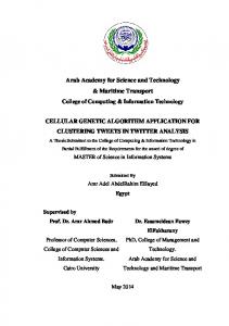
Fig. 2. Approximated fronts of aMOCell4, NSGA-II, and SPEA2 when solving WFG6

most important differences come out in the ZDT family, where the ∆ values of aMOCell4 in ZDT1, ZDT2 and ZDT6 are one order of magnitude lower than those reached by NSGA-II and SPEA2. In order to illustrate this fact, Fig. 2 displays the approximated WFG6 front of each algorithm which reported the best ∆ value out of the 100 trials. (We have chosen this MOP because it is one in which aMOCell4 is the best neither in GD nor in HV .) As it can be seen, aMOCell4 presents an almost perfect distribution of non-dominated solutions along the Pareto front, whereas some gaps exits in the fronts computed by NSGA-II and SPEA2. This is especially important when comparing aMOCell4 against NSGA-II, because they are implemented within the jMetal framework and hence they share the same ranking and crowding procedures. This shows the enhanced search capabilities of our cellular approach. The results of the HV metric are included in Table 9. As in the GD metric, aMOCell4 gets the best (now highest) values in ten out of the fourteen considered MOPs. It is clearly the best algorithm for the ZDT family and it reaches the best values in five out of the nine problems of the WFG toolkit (NSGA-II and SPEA2 are the best in two problems each). At this point, we want to remind the reader again that the small differences among the optimizers are because of the normalization process performed before calculating the metrics. However, these

small differences lead to discernible differences in the Pareto fronts, as shown in Fig. 2.

5

Conclusions and Future Work

In this work we have proposed and studied several issues in the design of MOCell in order to improve its performance. The basic MOCell algorithm is a multiobjective cGA which uses an external archive to store the non-dominated solutions found during the search. The studied design issues are related to the synchronicity in the update of individuals, the feedback from the archive, and the replacement policy. Six variants of MOCell have been compared using a standard methodology which is currently used in the evolutionary multiobjective optimization community. We have selected two benchmark of MOPs, the classical ZDT set of problems, usually used in similar studies in the area, and the recent benchmark obtained by using the WFG toolkit. Three metrics were used to assess the performance of the algorithms. The obtained results indicate that an asynchronous version, combined with replacing the worst cell in the neighborhood and using an individual from the archive in the selection operator leads to the best variant of the six analyzed versions of MOCell. To assess how competitive the most promising variant of MOCell is, we have compared it against two state-of-the-art evolutionary algorithms for solving MOPs, NSGA-II and SPEA2. The results of the comparison reveal that, in the context of the problems, the metrics, and the parameter settings used, aMOCell4 clearly outperforms the other two algorithms. A deeper study of MOCell, using problems of more than two dimensions, as well as an analysis of other design issues, such as different cell update strategies in the asynchronous versions, are matters for future work.

References 1. Deb, K., Pratap, A., Agarwal, S., Meyarivan, T.: A fast and elitist multiobjective genetic algorithm: NSGA-II. IEEE Trans. on Evol. Computation 6 (2002) 182–197 2. Knowles, J., Corne, D.: The pareto archived evolution strategy: A new baseline algorithm for multiobjective optimization. In: CEC 1999. (1999) 9–105 3. Zitzler, E., Laumanns, M., Thiele, L.: SPEA2: Improving the strength pareto evolutionary algorithm. Technical Report 103, Computer Engineering and Networks Laboratory (TIK), Swiss Federal Institute of Technology (ETH) (2001) 4. Jaeggi, D., Parks, G., Kipouros, T., Clarkson, J.: A multi-objective tabu search algorithm for constrained optimisation problems. In Coello, C., Hern´ andez, A., Zitler, E., eds.: EMO 2005. Volume 3410 of LNCS. (2005) 490–504 5. Nebro, A.J., Luna, F., Alba, E.: New ideas in applying scatter search to multiobjective optimization. In Coello, C., Hern´ andez, A., Zitler, E., eds.: EMO 2005. Volume 3410 of LNCS. (2005) 443–458 6. Alba, E., Tomassini, M.: Parallelism and Evolutionary Algorithms. IEEE Trans. on Evolutionary Computation 6 (2002) 443–462

7. Cant´ u-Paz, E.: Efficient and Accurate Parallel Genetic Algorithms. Kluwer Academic Publishers (2000) 8. Manderick, B., Spiessens, P.: Fine-grained parallel genetic algorithm. In: Proc. of the Third Int. Conf. on Genetic Algorithms (ICGA). (1989) 428–433 9. Whitley, D.: Cellular genetic algorithms. In Forrest, S., ed.: Proc. of the Fifth International Conference on Genetic Algorithms (ICGA), California, CA, USA, Morgan Kaufmann (1993) 658 10. Tomassini, M.: Spatially Structured Evolutionary Algorithms: Artificial Evolution in Space and Time. Natural Computing Series. Springer-Verlag, Heidelberg (2005) 11. Alba, E., Dorronsoro, B.: The exploration/exploitation tradeoff in dynamic cellular evolutionary algorithms. IEEE Trans. on Evol. Computation 9 (2005) 126–142 12. Alba, E., Dorronsoro, B., Giacobini, M., Tomasini, M.: Decentralized Cellular Evolutionary Algorithms. In: Handbook of Bioinspired Algorithms and Applications, Chapter 7. CRC Press (2006) 103–120 13. Laumanns, M., Rudolph, G., Schwefel, H.P.: A Spatial Predator-Prey Approach to Multi-Objective Optimization: A Preliminary Study. In: PPSN V. (1998) 241–249 14. Murata, T., Gen, M.: Cellular Genetic Algorithm for Multi-Objective Optimization. In: Proc. of the 4th Asian Fuzzy System Symposium. (2002) 538–542 15. Kirley, M.: MEA: A metapopulation evolutionary algorithm for multi-objective optimisation problems. In: CEC 2001, IEEE Press (2001) 949–956 16. Alba, E., Dorronsoro, B., Luna, F., Nebro, A., Bouvry, P., Hogie, L.: A Cellular Multi-Objective Genetic Algorithm for Optimal Broadcasting Strategy in Metropolitan MANETs. Computer Communications (2006) To appear 17. Grimme, C., Schmitt, K.: Inside a predator-prey model for multi-objective optimization: A second study. In Cattolico, M., ed.: GECCO-2006, Seattle, Washington, USA, ACM Press (2006) 707–714 18. Nebro, A.J., Durillo, J.J., Luna, F., Dorronsoro, B., Alba, E.: A cellular genetic algorithm for multiobjective optimization. In Pelta, D.A., Krasnogor, N., eds.: NICSO 2006. (2006) 25–36 19. Zitzler, E., Deb, K., Thiele, L.: Comparison of multiobjective evolutionary algorithms: Empirical results. IEEE Trans. on Evol. Computation 8 (2000) 173–195 20. Huband, S., Barone, L., While, R.L., Hingston, P.: A scalable multi-objective test problem toolkit. In Coello, C., Hern´ andez, A., Zitler, E., eds.: EMO 2005. Volume 3410 of LNCS. (2005) 280–295 21. Durillo, J.J., Nebro, A.J., Luna, F., Dorronsoro, B., Alba, E.: jMetal: A java framework for developing multiobjective optimization metaheuristics. Technical Report ITI-2006.10, Dpto. de Lenguajes y Ciencias de la Computaci´ on (2006) 22. Deb, K., Agrawal, R.: Simulated Binary Crossover for Continuous Search Space. Complex Systems 9 (1995) 115–148 23. Demˇsar, J.: Statistical comparisons of classifiers over multiple data sets. Journal of Machine Learning Research 7 (2006) 1 30 24. Deb, K.: Multi-Objective Optimization Using Evolutionary Algorithms. John Wiley & Sons (2001) 25. Van Veldhuizen, D.A., Lamont, G.B.: Multiobjective Evolutionary Algorithm Research: A History and Analysis. Technical Report TR-98-03, Dept. Elec. Comput. Eng., Air Force Inst. Technol. (1998) 26. Zitzler, E., Thiele, L.: Multiobjective Evolutionary Algorithms: A Comparative Case Study and the Strength Pareto Approach. IEEE Trans. on Evol. Computation 3 (1999) 257–271