A Novel Multi-Objective Genetic Algorithm for Product ...

Asia Pacific Industrial Engineering and Management System

A Novel Multi-Objective Genetic Algorithm for ProductMix Planning and Revenue Management for Semiconductor Fabrication Foundry Service *

Chen-Fu Chiena, Jei-Zheng Wub a

Department of Industrial Engineering & Engineering Management,National Tsing Hua University, Hsinchu 300, Taiwan b Department of Business Administration, Soochow University, Taipei 100, Taiwan

Abstract Semiconductor manufacturing is very capital intensive, in which matching the demand and capacity is the most important and challenging decision due to the long lead time for capacity expansion and shortening product life cycles of various demands. Most of previous works focused on capacity investment strategy or product-mix planning based on single evaluation criterion such as total cost or total profit. However, different combination of product-mix will contribute to different combination of key financial indicators such as revenue, profit, gross margin. This study aims to model the multi-objective product-mix planning and revenue management for the manufacturing systems with unrelated parallel machines. Indeed, the present problem is a multi-objective nonlinear integer programming problem. Thus, this study developed a multi-objective genetic algorithm for revenue management (MORMGA) with an efficient algorithm to generate the initial solutions and a Pareto ranking selection mechanism using elitist strategy to find the effective Pareto frontier. A number of standard multiobjective metrics including distance metrics, spacing metrics, maximum spread metrics, rate metrics, and coverage metrics are employed to compare the performance of the proposed MORMGA with mathematical models and experts’ experiences. The proposed model can help a company to formulate competitive strategy to achieve the first-priority objective without sacrificing other benefits. A case study in real settings was conducted in a leading semiconductor company in Taiwan for validation. The results showed that MORMGA outperformed the efficient multi-objective genetic algorithm, i.e., NSGA-II, in both revenue and gross margin. Keywords: PDCCCR; manufacturing strategy; multiple objectives; Pareto ranking; semiconductor manufacturing

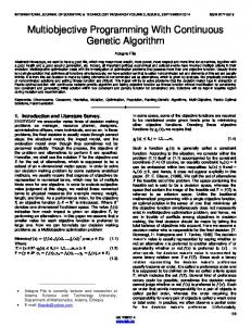
1. Introduction Following Moore’s law that the number of transistors fabricated on a wafer will be doubled every 12 or 24 months with lower average selling price [1], the new generation product will dominate prior generations regarding the cost-per-function. This technology migration will accelerate the price decline of prior generation products. The increasingly fierce competition also has commodified chip sales and led to continuous and significant price decline [2-3]. With continuously advanced functions with reducing average unit cost, semiconductor applications are continuously expanding and penetrating into various segments. Smart integrated circuits (ICs) have been increasingly employed in medical electronics, green energy, car electronics, computers, communication, and consumer electronics. In general, IC product demands can be categorized into logic ICs and memory ICs. Logics ICs are generally fabricated by wafer foundry companies whereas memory ICs are standard products and normally produced by integrated device manufacturers. Both semiconductor manufacturers are facing challenges to supply high variety of product by utilizing common and dedicated processes and machines. To respond to increasing demand, manufacturing strategic decisions of the interrelated determinants include Pricing strategies, Demand forecast and demand fulfillment planning (D), Capacity planning and capacity portfolio, Capital expenditure, and Cost structure that will affect the overall financial Return (R) of semiconductor manufacturing companies, as illustrated in the PDCCCR conceptual framework of Fig. 1 [4-6].

Fig. 1. Conceptual framework of PDCCCR (Chien et al. 2010a; Chien and Kuo, 2012)

Forecasts of future demands from various marketplaces provide the basis for capacity decisions. However, the demand fluctuation due to shortening product life cycle and increasing product diversification in the consumer electronics era make the demand forecast problem increasingly difficult and complicated. Demand forecast errors cause either inefficient capacity utilization or capacity shortage that will significantly affect the capital effectiveness and profitability of semiconductor manufacturing companies [4]. Conventional approaches for capacity management include capacity transformation and expansion investment from strategic level to operational level [7], new product allocation, intra-company inter- and intra-fab backup [8], inter-company backup [5], outsourcing [9-11], and productivity enhancement [12]. Most of the approaches have been applied by semiconductor manufacturing companies to meet diverse and increasing demands [13]. However, the capacity planning in the semiconductor industry can be characterized by high capital expenditure in capacity investment, long capacity installation lead times, high obsolescence rates due to rapid technology development, high demand volatility [7, 14]. Indivisibility, irreversibility, and nonconvexity in capacity cost modeling contribute to additional complexity of the problem [15]. Most of existing capacity planning models consider single return objective function such as cost, profit, utilization, or possibility of shortage [16-17]. Yet, the optimization of a single objective is solved at the expenses of other financial and operating indexes. For example, maximizing profitability may lead to the loss of market share due to abandon of low-profit-margin-but-high-volume demand. This study aims to propose a multi-objective capacity planning model to address the product-mix, process and backups among different product families and technologies to maximize the synergistic benefits of revenue growth, profitability, and wafer outputs, which are critical to evaluate the competitiveness of a semiconductor company. Without loss of generality, the aforementioned model lies in the category of quantity-based revenue management decisions comprising allocations of output or capacity to different segments, products or channels [19-20]. To deal with the nature of high combinatorial problem complexity involved in the present problem, this study developed an efficient multi-objective revenue management genetic algorithm (MORMGA). For validation, this study conducts comparisons among multi-objective genetic algorithms and their settings. Standard multiobjective performance metrics such as distance metrics, spacing metrics, maximum spread metrics, rate metrics, and coverage metrics are employed. Decision makers can select the beneficial alternatives of product-mix and capacity configuration decisions from a set of nondominated solutions without the need of a priori articulation of preferences among multiple objectives. The remainder of this paper is organized as follows. Section 2 defines the multi-objective productmix planning and revenue management for the semiconductor manufacturing systems with unrelated parallel machines and proposes a mathematical model to find exact solution of the problem. Section 3 proposes an efficient multi-objective genetic algorithm model to solve the problem. Section 4 examines the proposed genetic algorithm with real case data. Section 5 concludes with discussions of contributions and future research directions. 2. Problem Definition 2.1. Assumptions (1) Inventory and backlog are not considered. This study focused on semiconductor wafer fabrication

foundry service that is make-to-order without inventory, while backlog will become deferred demand [8]. (2) All parameters are known and constant. There are two important reasons to show why deterministic models are reasonable. Firstly, deterministic models are easy to analyze and can serve as a good approximate for the more realistic yet complicated stochastic models. Deterministic solutions are asymptotically optimal for the stochastic demand problem in some cases. Secondly, deterministic models are more applicable in practice [18]. (3) Prices, cost structures, and demand forecasts are given. This study focused on quantity-based revenue management models, i.e. capacity allocation and configuration [19-20]. The proposed model can be further applied for examining different pricing strategies, cost management plans, and demand scenario analysis. (4) Large-scale capacity expansion decision is formed in advance, and is thus not considered in this model. This problem focused on short-term capacity configuration and allocation decisions. 2.2. Functions

 x   x  [ x]



- Ceiling of x is the smallest integer not less than x - Floor of x is the largest integer not greater than x -

 max( x , 0)

2.3. Superscripts and subscripts b g h i k, m n r

-

product type demand group machine area group order item machine group number of layers machine recipe

2.4. Sets m

B G Gi

I b I Ig

- set of product groups that can be processed on machine group m - set of demand groups - set of demand group that order i belongs to - set of orders - set of orders that belong to product type b - set of orders that belong to product group g

J

- set of machine area groups - a sequence of pair machines [(k , m ) (k , m ) ... (k , m )] that can be exchanged from one to 1 1 2 2 |K | |K|

Κ

another. The pair machines are sorted in the increasing order of Fkm / Vkm - a sequence of machine groups that is sorted in the increasing order of Fm / Vm

M h

M Mb

- set of machine groups that belong to area group h - set of machine groups where product group b will be processed on

N

bm

- set of process layers where product group b will be processed on machine group m

R

bmn

- set of recipe by which product group b will be processed on machine group m through layer n

2.5. Parameters

Bi

- average availability of machine group m - product type of order i

Cb

- variable cost of product type b

Am

Di

- unit cost per hour for additional direct labor hours - max demand of order i

Di

- minimum (committed) demand of order i. Without loss of generality, D min  D max . i i

Di

- range of demand of order i, specifically D range  D max  D min  0 i i i

Em

- efficiency of machine group m. - total capacity expansion budget of the planning horizon - capital expenditure of machine group m written down within the planning horizon - unit cost of exchange from machine group m to machine group k

CDL max

min

range

F Fm Fmk

Gg

- fixed cost - maximum output of demand group g

Gg

- minimum output of demand group g

H

- total hours within the planning horizon - net available capacity of machine group m within the planning horizon - unit loading of order item i when processed machine group m

G max

min

Hm H im

Km

- unit loading of product group b when processed on the nth layer by using machine group m with recipe r - area group attribute of machine group m - indicating whether machine group m needs to be operated by direct labors

Oj

- max number of machine area group j that can be acquired

Pi

- unit price of product item i - maximum number of machine group m acquired within the planning horizon

H bmnr Jm

Qm

max

Rbmnr S

S bmnr Vm Vkm

- rework rate of product group b when processed on the nth layer by using machine group m with recipe r - the number of steps that the current direct labor level can support - number of steps of product group b when processed on the nth layer by using machine group m with recipe r - capacity ramping-up rate of acquiring machine group m - capacity exchange rate of exchanging from machine group k to machine group m

Wbmr

- equivalent output of product item i - wafer-per-hour throughput of product type b processed on machine group m using recipe r

Ybmnr

- yield rate of using machine group m to process product type b on the nth layer

Wi

2.6. Decision variables xi

- capacity supported demand (CASD) of order i

qm

- number of machine group m acquired within the planning horizon

q km

- capacities exchanged from machine group k to machine group m

2.7. Objective functions and constraints max z REV 

 Px i

(1)

i

iI

 Px   C  x   i

max z MAR 

iI

i

b

bB

i

iI

b

Fkm qkm  Fm qm  G  CDL [

( k , m )K

K 

 iI

Px i i



H im xi  S ]

m

mM

m

bB , iI

b

(2)

W x

max zOUT 

i

(3)

i

iI

Gg

min



x

 G g , g  G max

i

(4)

iI g



H im xi  H m  Vm q m 

m

b  B , i I

q mM

b



Vkm q km 

( k , m ) K



qmk , m  M

(5)

( m , k ) K

 Oh , h  H

m

(6)

h

F q m

F

m

(7)

mM

 xi  Di , i  I

(8)

qm  {0,1, 2,..., Qm }, m  M

(9)

Di

min

max

max

q km  0,  ( k , m )  K

(10)

Where H m  H  Am  E m , m  M

(11)

H bmnr  H im 

S bmnr WPH bmr (1  Rbmnr )Ybmnr

H nN

bm

r R

bmn

, m  M , b  B , n  N , i  I , r  R m

, m  M , b  B , i  I m

bmnr

bm

b

bmn

(12)

b

(13)

The objective of the proposed (these two terms combined may be confusion) model is to simultaneously achieve three non-commensurable objectives including revenue maximization in Eq. (1), profit margin maximization in Eq. (2), and equivalent output in Eq. (3). The formulation in Eq. (2) entails treatment to nonlinearity that also justifies the use of genetic algorithm in which the direct labor costs are evaluated when modeling product-mix planning. The decision model is bounded by strategic constraints (Eq., 4) that revealed long-term vision for the company and considered competitors’ actions as discussed in [21]. One reminding example was Intel’s decision on retiring commoditized memory products that could benefit Intel with economies of scales while the beginning of microprocessor products had no advantage regarding marginal profit per unit of capacity supplied. In this case, minimum demand for microprocessor products and maximum demand of memory products shall be considered. Setting up the floor of grouping demand for ramping-up new technology and ceiling for old technology is another common strategic constraint. Capacity allocation and configuration constraints are formulated in Eq. (5) to show the relationship between machine requirement and machine supply by considering the number of steps, throughput rate, rework rate, yield rate, machine hours, number of machines on hand, number of incremental machines, number of planned retrofits, number of retrofits to be done, machine availability, and efficiency as detailed from Eq. (11) to Eq. (13). The effective capacity will consider the loss rates during ramping-up and retrofitting. In semiconductor wafer fabrication, a product will go through complex operations of multi-layer process which comprise a number of machine groups. The portion of convertible machine groups for capacity requirement may differ among different operations. Capacity requirement of different machine groups for each product group may also differ in each operation. A machine group can be characterized by its capability of processing multiple product groups. In particular, a dedicated machine group can support only one product group whereas different product groups may share capacity on a machine group. In addition, convertible machine groups can be converted to support different product groups with additional loss on cost and capacity. A machine group can be further characterized by its process technology. Old technology cannot be employed to produce advanced products. There are three ways of increasing capacity for a machine group: acquisition and backup (exchange). By acquisition, a new machine group can be purchased, installed, and ramped up to support future demand. By exchange, when the working time of common tools allocated to a technology increases, the capacity will increase accordingly. Constraints (6) and (7) specify the limitations of facility spaces (enclosed by the building, land clean room floor space, machine types, categories of manpower, etc.) [22] and annual budget for small-scale expansions, respectively. Constraint (8) defined the boundary of demands. Finally, equations (9) and (10) show nonnegative integer variables for machine acquisition, and retrofit, respectively.

 Px

max z REV 

i

(14)

i

iI  M

H ii x i  Vi q i ,  i  I  M

(15)

 Fq

(16)

i

i

F

iI  M

H ii xi  Vi qi , i  I  M

(17)

qi  {0,1, 2, ..., Qi }, i  I  M

(18)

max

max z REV 

 Px   ( PV / H i

iI  M

i

i

i

ii

) qi

i  mI

(19)

The aforementioned mathematical model is computationally intractable, especially when the problem size increases significantly. Considering the special case where each order item requires distinct and unique tool to process, the single-objective problem (14) subject (15)-(19) is a bounded Knapsack problem, a NP-hard (non-deterministic polynomial) problem [23]. Generally speaking, multiobjective optimization problems were more difficult [24]. Approaches to tackle multi-objective optimization problems can be categorized as priori, interactive, and posteriori ones according to the timing when decision-makers’ preferences were introduced [25-27]. Priori approaches can be transformed to single-objective optimization problems by using weighting or lexicographic methods. However, it is inefficient and hard to elicit decision-makers’ preferences when no alternatives are provided in the dynamic planning environment. Interactive methods are neither efficient nor cost-effective when the design spaces are wide-spread in the planning problem. Alternatively, after a limited number of solutions are specified through a posteriori approach, it can be transformed to transform it to an interactive approach to elicit decision-makers preferences on alternatives when corresponding criterion values are determined [28]. Multi-objective genetic algorithms are relatively effective to find the nondominated (Pareto) solution set. In particular, a number of tests on NSGA-II with and without constraint dominances showed its efficiency on solving multi-objective optimization problems with continuous variables [29]. However, the lack of empirical experiments on multi-objective combinatorial problems limits its application to product-mix and capacity configuration planning problems. Added to this, the elitism strategy does not guarantee diversity of nondominated solutions. 3. Multiple-Objective Revenue Management Genetic Algorithm This study modifies the NSGA-II with constraint handling [29] to develop a multi-objective genetic algorithm (MORMGA) to solve the product-mix and revenue management problem with revenue maximization, profit margin maximization, and equivalent output maximization objectives. MORMGA consider five parameters including generation size (Ng), population size (Np), global front size (Ns), crossover rate (rp), and mutation rate (rm). The generation, denoted by t, represents the number of computation iterations of the GA. It contains Np chromosomes and corresponding solutions that collectively represents a population, denoted as P(t). Initial chromosomes are randomly generated. The crossover rate represents the ratio of the number of offspring produced in each generation to the population size, whereas the mutation rate represents the percentage of the total number of chromosomes in the population. The global Pareto solutions can be updated at each generation after the NSGA-II process (Fig. 2). The newly generated Pareto solutions are those with rank one. However, these solutions should be compared with the existing Pareto solutions, since there is no guarantee of non-dominance when the two sets are pooled. One point in the new set can be dominated by another point in the old set, while one point in the old set can be dominated by another point in the new set. It is possible to pool the two sets into a single population, and then adopt the NSGA-II to find the updated Pareto solutions. A bi-vector encoding method is embedded in the proposed MORMGA. An allocation vector A = [α1 α2 … α|I|] contains genes that represent the percentage of individual orders to be allocated. The value of each gene, namely genotype, is encoded as a random key [30]. For example, given an order item i in I ୰ୟ୬୥ୣ with gene αi in [0,1], the corresponding allocation is ‫ݔ‬௜ ؔ ‫ܦ‬௜୫୧୬ ൅ ߙ௜ ‫ܦ‬௜ . The other vector B = [β1 β2 …β|I|] is a permutation of [1 2 … |I|] that contains genes representing the sequence of individual orders to be allocated. The lengths of both vectors equal the number of orders, i.e. |I|.

procedure: multi-objective revenue management genetic algorithm (MORMGA) begin initialize P(t) evaluate P(t) based on the proposed decoding method generate global Pareto solutions by inserting the rank-one solutions with zero penalty value for t = 1 to Ng do recombine P(t) to yield O(t) by using the two cut-point crossover and the partition randomization mutation for the allocation vector (random key-based representation) and the partition mapping crossover and the insertion mutation for the sequence vector (permutation-based representation) [11] evaluate O(t) based on the proposed decoding method and the NSGA-II [29] R (t )  P (t )  O(t ) - combine parent and offspring population R  {R 1 , R 2 , ...}  fast-non-dominated-sort( R ( t )) - sort nondominated fronts of R (t )

P (t  1)   and i  1

while | P(t  1) |  | R i | N p do - until the parent population is filled P ( t  1)  P ( t  1)  R i - include ith nondominated front in the parent population

i : i  1 - check the next front for inclusion Apply crowding-distance-assignment, i.e. D C ( a ),  a  R i - calculate crowding distance in R i

P(t  1)  P(t  1)  R i [1: ( N p  | P(t  1) |)] - the first ( N p  | P (t  1) |) elements of R i Sort( R i , C ) - sort in descending order using revised crowded-comparison operator ( C ): a C b if a is of zero penalty but b is not

or {it not the reverse case that b is of zero penalty but a is not and [ a  b (week dominance with respect to objective values) or ( a  b (non-dominance) and DC ( a )  DC (b ) (using crowding distance))]} U  S (t ) - initialize the joint global Pareto front for u  P(t  1) do if the penalty objective of u is not zero then next u - update with feasible solutions only U  U  {u} - initialize the joint global Pareto front for v  S(t ) do if u  v then U  U \ {v} - check whether v is dominated

else if u  v then U  U \ {u} and next u - check whether u is dominated Apply crowding-distance-assignment( U ) - calculate crowding distance in U Sort(U , C ) - sort U in descending order of crowding distance S (t  1)  U[1 : N s ] - choose the first N s elements of U t  t 1

end Fast-Non-DominatedSorting (FNDS)

Revised Crowding Distance Sorting

Global Front Update

R1

P(t )

Revised Crowding Distance Sorting

S(t )

Ns

R2

S(t  1)

Np R3

P(t  1)

U(t )



O(t )



Rejected R (t )

Constraint-handling: zero-penalty solution has higher priority

Fig. 2. Multi-objective revenue management genetic algorithm (MORMGA), a revised NSGA-II procedure

procedure: decoding method (a local search) input (including parameters and variables mentioned in the mathematical model) Α : An allocation chromosome [1  2  |I| ] A sequence chromosome [ 1  2  |I| ]

Β: output Α:

A repaired allocation chromosome c, qm , m  M , and qkm , ( k , m)  K : Three sets of decision variables z REV , z MAR , z OUT , and z PEN : Three objective values and one penalty value ( z PEN ) that sums overall

exceeding loading. begin   i Di

xi  Di

min

range

, i  I

 g   xi , g  G , denotes output of demand group g iI g

Apply procedure: prior-repair method to meet strategic demand group constraint Apply procedure: capacity allocation and reconfiguration method Apply procedure: post-repair method to meet capacity constraints and to improve tool utilization z REV 

 Px i

i

i I

 Px   C  x   i

z MAR 

i

b

iI

bB

i

iI

b

Fkm qkm  Fm qm  G  CDL [

( k , m )K

K 

 Px i



H im xi  S ]

m

mM

m

bB , iI

b

i

iI

z OUT 

W x i

i

iI

z PEN 



m

m M ,  m  0

end procedure: prior-repair method to meet strategic demand group constraint input (including parameters and variables mentioned in the mathematical model) Α : An allocation chromosome [1  2  |I| ]

Β:

A sequence chromosome [ 1  2  |I| ]

Ν:

A vector [ 1 2  |G| ] denoting outputs of demand groups

X:

A vector [ x1 x2  x|I| ] denoting capacity supported demand (CASD) of orders

output Α : A repaired allocation chromosome Ν : A repaired vector denoting outputs of demand groups X : A repaired vector denoting capacity supported demand (CASD) of orders begin for j  1 to | I | where i   j and  i  1 do  i  min{[max(Gg   g )] , (1   i ) Di 

min

range

g G i

} , denotes the increment

g  g  i , g  Gi  i   i  i / Di

range

xi  xi   i

for

j | I | to 1 where i   j and i  0 do  i  min{[max(  g  G g )] , min(  g  Gg ),  i Di max

g G i



min

g G i

range

} , denotes the reduction

g  g  i , g  Gi  i  i  i / Di

range

xi  xi   i

end procedure: capacity allocation method input (including parameters and variables mentioned in the mathematical model) X : A vector [ x1 x2  x|I| ] denoting capacity supported demand (CASD) of orders output qm , m  M , and qkm , ( k , m)  K : Two sets of capacity-related decision variables

Ρ:

A vector [ 1 2  |M| ] denoting loadings of each tool group

:

A vector [1 2  |M| ] denoting exceeding loadings

begin

m 

 m

H im xi , m  M

bB , iI

b

 m   m  H m , m  M q m  0, m  M qkm  0, ( k , m )  K

  F , denotes remaining budget for tool acquisition   O , j  J , denotes remaining quota for installing tools in area j F

j

j

for a  1 to | K | where ( k , m)  ( k a , ma ) ,  k  0 , and  m  0 do q km  min(  k ,  m / Vkm ) , denotes the maximum capacities that can be exchanged from tool k

to tool m without sacrificing those orders which tool k can originally support  m   m  Vkm qkm  k   k  qkm

for m  1 to | M | where  m  0 do j  Jm

qm  min( m / Vm  , Qm ,  / Fm  ,  j ) , denotes the maximum number of tool to be acquired  m   m  Vm qm max

F

    Fm qm F

F

 j   j  qm for a  1 to | K | where ( m, n)  ( k a , ma ) ,  m  0 , and  n  0 do q mn  min(  m ,  n / Vmn ) (incremental tools may yield surplus capacities that can

support others)  n   n  Vmn qmn  m   m  qmn

end procedure: post-repair method to meet capacity constraints and to improve tool utilization input (including parameters and variables mentioned in the mathematical model) Α : An allocation chromosome [1  2  |I| ]

Β:

A sequence chromosome [ 1  2  |I| ]

Ν:

A vector [ 1 2  |G| ] denoting outputs of demand groups

X:

A vector [ x1 x2  x|I| ] denoting capacity supported demand (CASD) of orders

Ρ:

A vector [ 1 2  |M| ] denoting loadings of each tool group

:

A vector [1 2  |M| ] denoting exceeding loadings

output Α : A repaired allocation chromosome Ν : An updated demand group output vector X : An updated CASD vector Ρ : An updated loading vector  : An updated exceeding loading vector begin for j | I | to 1 do i   j and b  Bi

 i  min{min(  g  Gg ),  i Di min

range

g G i



,[max( m / H im )] } mM b

//  i denotes the order quantity reduction to solve the problem of overloading

g  g   i , g  Gi i   i   i / Di

range

xi  xi   i  m   m  H im i , m  M b

 m   m  H im i , m  M b for j  1 to | I | do i   j and b  Bi

i  min{min(Gg   g ), (1   i ) Di max

g G i

range



,[min(  m / H im )] } mM b

// i denotes the order quantity increment to solve the problem of low utilization

g  g  i , g  G i i  i  i / Di

range

xi  xi  i  m   m  H imi , m  M b

 m   m  H imi , m  M b end 4. Numerical Results with Real Settings

The proposed MORMGA was examined in a wafer fabrication foundry company located in Hsinchu Science Park of Taiwan. To ensure confidentiality, data was transformed by reserving comparative results without loss of generality for further explanation. The data comprised 10 products and 72 tool functions. Total product route were 2847 steps, each product had to go through an average about 300 steps. In the same data, three pairs of backups are provided. Three working areas spared extra space for small-scale tool acquisition. The annual investment limit was $ 200 million and direct-labor move limit was 198 million steps. More details are elaborated in tables A1 to A5 of Appendix. To evaluate and compare multi-objective optimization algorithms, this study adopted conventional performance metrics including the relative average distance (Dav) to the reference front, the percentage of range that the solution set covers the reference front (MS), the space metric used to measure how

evenly the solutions are distributed (Tan’s spacing, TS), the rate metric (R), coverage metric (C), and running times (RT) [31-32]. Four numerical tests were performed. Designs of the MORMGA were firstly evaluated. The best MORMGA design was applied thereafter. Secondly, effectiveness of backup and acquisition was examined and compared. After that, complexity effects were evaluated based on four different size problems with the same problem structures. Finally, full-scale test results were presented. Numerical analysis was performed on a desktop computer equipped with an Intel® Core™ Quad CPU Q8400 @ 2.66GHz and 3.25GB RAM. The commercial software LINGO 11.0 (LINGO System) was used to generate a reference set of non-dominated solutions by utilizing embedded integer programming (IP) packages. LINGO solved the weighted-sums problem with objectives (1)-(3) subject to (4)-(10) a number of enumerative weight settings. Each problem instance was recognized as “nonlinear integer linear programming” (NILP) and terminated at local optimal solutions. A local optimal solution was collected within various ranges of computation time. Accordingly, a set of reference non-dominated solutions were generated for evaluation purpose. The benchmark mathematical programming solutions were denoted by MONLP hereafter. The nondominated solutions generated by MONLP were used as reference fronts for aforementioned multi-objective metric calculations. All test ran set generation size Ng = 2,000 and population size Np = 50. Each algorithm design for comparison was the combination of a candidate selection methods and a setting of global front size (Ns). Selection methods included (A) rNSGA-II (the NSGA-II with constrained dominance), (B) NSGA-II (NSGA-II without constrained dominance), (C) exponential ranking roulette wheel selection with multiplier equal to 0.5 [33], and (D) linear ranking roulette wheel selection [34]. Options of the length of tacking list comprised (a) unlimited, (b) 200, (c) 50, and (d) none. Each combination ran 10 replications. Note that the combination A-b represents the proposed MORMGA with Ns = 200 whereas A-d is the conventional constraint-handling NSGA-II. The numerical results showed that selection methods and the global front sizes are determinants to computational performances (significance level = 0.001) (Fig. 3 to Fig. 6). Yet, the choices between constrained dominance or not made little differences. Although unlimited number of global fronts outperformed in most of the indexes, it was one of the sources of computational complexity. The decision-makers should perform careful trade-off between solution quality and computational times on the choices of Ns. The following analysis applied rNSGA-II with the global front size Ns = 200. Main Effects Plot (data means) for MS

Main Effects Plot (data means) for Dav method

track

method

0.95

0.050

track

0.90

0.045

Mean of MS

Mean of Dav

0.85 0.040 0.035 0.030

0.80 0.75 0.70

0.025

0.65 0.60

0.020 A

B

C

D

a

b

c

d

Fig. 3. Results of Davs (lower is better)

A

C

D

a

b

c

d

Fig. 4. Results of MSs (higher is better) Main Effects Plot (data means) for R

Main Effects Plot (data means) for TS method

0.12

B

track

method

1.0

track

0.9

0.10

Mean of R

Mean of TS

0.8 0.08 0.06

0.7 0.6 0.5

0.04

0.4 0.02

0.3 0.2

0.00 A

B

C

D

a

Fig. 5. Results of TSs (lower is better)

b

c

d

A

B

C

D

a

b

c

d

Fig. 6. Results of Rs (higher is better)

From the multi-objective perspective, this study proposed a comparison scheme for analyzing the effectiveness of backup and acquisition. Four cases for comparisons were designed as shown in table 1.

Particularly, the case IV was the test problem discussed in the previous section. The case I expressed the situation when neither backup nor acquisition is permitted. Cases II and III represented the situations when merely backup or acquisition is allowed, respectively. Without the option of acquisition, the cases I and II are formulated as multi-objective fractional linear programming models. The complexity sequence of the cases in ascending order is I, II, III, and IV. The result showed that the running times of proposed MORMGA had little differences among all cases even though theoretically cases III and IV were harder than cases I and II (Fig. 7). On the other hand, the running times of cases I, II, III, and IV on MONLP were 563, 601, 640, and 732 seconds, respectively. Case IV took 30% more computational time than case I by using MONLP, i.e., 100%× (732-563)/563. Regarding the solutions performance, the values of the rate metric increased as the generation size or the population size increased (Fig. 8). More explorations and more computation times could improve the solutions quality. Almost all values of the rate metric approach one. The Pareto fronts generated by MORMGA were close to the idea fronts. In addition, the low Tan’s spacing values showed that the solutions on the Pareto fronts of MORMGA were diversely distributed (Fig. 9). Table 1. Design for backup and acquisition comparisons

Backup

Case

No I III

No Yes

Acquisition

Yes II IV

800 700 600 500 400 300 200 100

500 1000 1500 2000 500 1000 1500 2000 500 1000 1500 2000 500 1000 1500 2000 500 1000 1500 2000 500 1000 1500 2000 500 1000 1500 2000 500 1000 1500 2000 500 1000 1500 2000 500 1000 1500 2000 500 1000 1500 2000 500 1000 1500 2000 500 1000 1500 2000 500 1000 1500 2000 500 1000 1500 2000 500 1000 1500 2000

0

50

100

150

200

50

100

I

150

200

50

100

II

150

200

50

100

III

150

200

IV

Fig. 7. Running Times of Cases I~IV

1.00 0.99 0.98 0.97 0.96 0.95 0.94 0.93 0.92 0.91

500 1000 1500 2000 500 1000 1500 2000 500 1000 1500 2000 500 1000 1500 2000 500 1000 1500 2000 500 1000 1500 2000 500 1000 1500 2000 500 1000 1500 2000 500 1000 1500 2000 500 1000 1500 2000 500 1000 1500 2000 500 1000 1500 2000 500 1000 1500 2000 500 1000 1500 2000 500 1000 1500 2000 500 1000 1500 2000

0.90

50

100

150

200

50

I

100

150

200

50

II

150 III

R(.)

Fig. 8. Rate Metrics of Cases I~IV

100

200

50

100

150 IV

200

0.03

0.02

0.01

500 1000 1500 2000 500 1000 1500 2000 500 1000 1500 2000 500 1000 1500 2000 500 1000 1500 2000 500 1000 1500 2000 500 1000 1500 2000 500 1000 1500 2000 500 1000 1500 2000 500 1000 1500 2000 500 1000 1500 2000 500 1000 1500 2000 500 1000 1500 2000 500 1000 1500 2000 500 1000 1500 2000 500 1000 1500 2000

0.00

50

100

150

200

50

I

100

150

200

50

II

100

150 III

200

50

100

150

200

IV

TS(.)

Fig. 9. Tan’s Spacing of Cases I~IV

5. Conclusions

This study developed the MORMGA to model and to solve the product-mix and revenue management problem for semiconductor manufacturing. The proposed model can help a company to formulate competitive strategy to achieve the first-priority objective without sacrificing other benefits. A GA parameter, the global frontier size, is introduced to provide a number of nondominated solutions for top management to make the final decision. There exists a trade-off between computation efficiency and the number of solutions to evaluate in the light of the quality of the solutions. The convergence and diversity of nondominated solutions are ensured, with satisfactory efficiency for implementation in real settings. Indeed, the proposed MORMGA can serve as a core computation engine of a decision support system for both demand and capacity planners without the need of a priori articulation of preferences among multiple objectives. Decision makers can select the beneficial alternatives of product-mix and capacity decisions from a set of nondominated solutions. However, a large number of solutions will delay decision-making lead times. In some cases, decision makers may jump into conclusions to prevent from trapping in the complex and lengthy discussions. To enhance decision-making quality, further research can be done in the area of finding efficient interactive models to articulate preferences from a set of nondominated solutions. Acknowledgements

This work was supported by National Science Council (NSC100-2410-H-031-011-MY2; NSC-1002628-E-007-017-MY3). References [1] Moore GE. Cramming more components onto integrated circuits. Electronics 1965; 38(8):114–17. [2] Chien C-F. (2007). Made in Taiwan: Shifting paradigms in high-tech industries. Industrial Engineer: IE, 39(2):47–9. [3] Chien C-F, Dauzère-Pérès S, Ehm H, Fowler JW, Jiang ZB, Krishnaswamy S, Lee T-E, Mönch L, Uzsoy R. Modeling and analysis of semiconductor manufacturing in a shrinking world: challenges and successes. European Journal of Industrial Engineering 2011; 5(3):254–71. [4] Chien C-F, Chen, Y-J, Peng, J-T. Manufacturing intelligence for semiconductor demand forecast based on technology diffusion and product life cycle. International Journal of Production Economics 2010; 128(2):496–50. [5] Chien C-F, Kuo, R-T. Beyond make-or-buy: Cross-company short-term capacity backup in semiconductor industry ecosystem. Flexible Services Manufacturing Journal 2013; 25(3):310–42. [6] Chien C-F, Zheng J-N. Mini-max regret strategy for robust capacity expansion decisions in semiconductor manufacturing. Journal of Intelligent Manufacturing 2012; 23(6):2151–59. [7] Wu SD, Erkoc M, Karabuk S. Managing capacity in the high-tech industry: A review of literature. The Engineering Economist 2005; 50(2), 125–58. [8] Chien C-F, Wu J-Z, Wu C-C. A two-stage stochastic programming approach for new tape-out allocation decisions for demand fulfillment planning in semiconductor manufacturing. Flexible Services and Manufacturing Journal 2013; 25(3):286–309.

[9] Chien C-F, Wu J-Z, Weng, Y-D. Modeling order assignment for semiconductor assembly hierarchical outsourcing and its decision support system. Flexible Services and Manufacturing Journal 2010; 22(1-2):109–139. [10] Wu J-Z, Chien C-F. Modeling strategic semiconductor assembly outsourcing decisions based on empirical settings. OR Spectrum 2008; 30(3):401–30. [11] Wu J-Z, Chien C-F, Gen M. Coordinating strategic outsourcing decisions for semiconductor assembly using a bi-objective genetic algorithm. International Journal of Production Research 2012; 50(1):235–60. [12] Leachman RC, Ding SW, Chien C-F. Economic efficiency analysis of wafer fabrication. IEEE Transactions on Automation Science and Engineering 2007; 4(4):501–12. [13] Shih W, Chien C-F, Shih C-T, Chang J. The TSMC way: Meeting customer needs at Taiwan Semiconductor Manufacturing Co, Harvard Business School Case Study 2009; 9-610-003. [14] Wu J-Z. Inventory write-down prediction for semiconductor manufacturing considering inventory age, accounting principle, and product structure with real settings. Computers & Industrial Engineering 2013; 65(1):128–36. [15] van Mieghem JA. Capacity management, investment, and hedging: Review and recent developments. Manufacturing & Service Operations Management 2003; 5(4):269–302. [16] Chen Z-L, Li S, Tirupati D. A scenario-based stochastic programming approach for technology and capacity planning. Computers and Operations Research 2002; 29(7):781–806. [17] Hood SJ, Bermon S, Barahona F. Capacity planning under demand uncertainty for semiconductor manufacturing. IEEE Transactions on Semiconductor Manufacturing 2003; 16(2):273–80. [18] Bitran G, Caldentey R. An overview of pricing models for revenue management. Manufacturing & Service Operations Management 2003; 5(3):203–30. [19] Talluri KT, van Ryzin GJ. The Theory and Practice of Revenue Management, NY: Kluwer Academic Publishers; 2004. [20] Talluri KT, van Ryzin GJ, Karaesmen IZ, Vulcano GJ. Revenue management: Models and methods. Proceedings of the 40th Winter Simulation Conference 2008; Dec. 11-14, Phoenix, Arizona. [21] Burgelman RA. Fading memories: A process theory of strategic business exit in dynamic environments. Administrative Science Quarterly 1994; 39(1):24–56. [22] Çakanyildirim M, Roundy RO, Wood SC. Optimal machine capacity expansions with nested limitations under stochastic demand. Naval Research Logistics 2004; 51(2):217–41. [23] Martello S, Toth P. Knapsack Problems: Algorithms and Computer Implementation, New York: John Wiley & Sons Ltd; 1990. [24] Marler RT, Arora JS. Survey of multi-objective optimization methods for engineering. Structural and Multidisciplinary Optimization 2004; 26(6):369–95. [25] Katagiri H, Sakawa M, Kato K, Nishizaki I. Interactive multiobjective fuzzy random linear programming: Maximization of possibility and probability. European Journal of Operational Research 2008; 188(2):530–39. [26] Molina J, Santana LV, Hernandez-Diaz AG, Coello Coello CA, Caballero R. g-Dominance: Reference point based dominance for multiobjective metaheuristics. European Journal of Operational Research 2009; 197(2):658–92. [27] Zio E, Bazzo R. A clustering procedure for reducing the number of representative solutions in the Pareto Front of multiobjective optimization problems. European Journal of Operational Research 2011; 210(3):624–34. [28] Ehrgott M, Gandibleux X. A survey and annotated bibliography of multiobjective combinatorial optimization. OR Spectrum 2000; 22(4):425–60. [29] Deb K, Pratap A, Agarwal S, Meyarivan T. A fast and elitist multiobjective genetic algorithm: NSGA-II. IEEE Transactions on Evolutionary Computation 2002; 6(2):182–97. [30] Bean JC. Genetic algorithms and random keys for sequencing and optimization. INFORMS Journal on Computing 1994; 6(2):154–60. [31] Li BB, Wang L, Liu B. An effective PSO-based hybrid algorithm for multi-objective permutation flow shop scheduling. IEEE Transactions on Systems, Man and Cybernetics - Part A: Systems and Humans 2008; 38(4):818–31. [32] Tan KC, Goh CK, Yang YJ, Lee TH. Evolving better population distribution and exploration in evolutionary multi-objective optimization. European Journal Operational Research 2006; 171(2):463–95. [33] Michalewicz Z. Genetic Algorithms + Data Structures = Evolution Programs, 3rd edition, New York: Springer; 1996. [34] Reeves C. A genetic algorithm for flow shop sequencing. Computers and Operations Research 1995; 22(1):5–13.

Appendix A. Raw Data for Analysis Table A1. Product information Product Technology Unit Price P01 I 17,400 P02 I 0 P03 I 14,500 P04 I 0 P05 II 8,700 P06 II 0 P07 II 11,600 P08 III 15,950 P09 III 17,400 P10 III 0

Var. Cost 4,350 4,350 4,060 4,060 3,480 3,480 2,871 2,900 3,770 3,770

Note: P02, P04, P06, and P10 are R&D engineering orders

Min. Qty 0 300 0 300 0 300 0 0 0 300

Max. Qty 7,000 300 7,000 300 3,000 300 3,000 9,000 9,000 300

Table A2. Tool information Cost Avail. Avail. Tool Area K/M Time Eff. T01 A 1 0.98 0.82 T02 A 1 0.98 0.82 T03 A 1 0.92 0.85 T04 A 1 0.96 0.93 T05 B 1 0.97 0.92 T06 C 1 0.97 0.92 T07 D 1 0.89 0.87 T08 A 1 0.94 0.86 T09 A 1 0.90 0.87 T10 B 1 0.93 0.94 T11 B 0 0.99 0.92 T12 C 1 0.91 0.96 T13 C 1 0.91 0.96 T14 C 1 0.93 0.93 T15 A 1 0.87 0.85 T16 A 1 0.87 0.85 T17 D 1 0.90 0.90 T18 A 1 0.87 0.93 T19 A 1 0.87 0.93 T20 A 1 0.87 0.93 T21 A 1 0.91 0.87 T22 D 0 0.95 0.92 T23 A 1 0.95 0.90 T24 C 1 0.95 0.96 T25 A 1 0.98 0.92 T26 A 1 0.77 0.87 T27 A 1 0.80 0.87 T28 A 1 0.72 0.87 T29 B 1 0.83 0.92 T30 A 1 0.92 0.87 T31 A 1 0.92 0.87 T32 D 1 0.84 0.89 T33 A 1 0.83 0.87 T34 A 1 0.97 0.82 T35 D 1 0.87 0.90 T36 B 1 0.92 0.94 T37 B 1 0.89 0.94 T38 B 1 0.92 0.94 T39 B 1 0.92 0.94 T40 B 1 0.93 0.94 T41 B 1 0.92 0.94 T42 B 1 0.91 0.93 T43 B 1 0.88 0.94 T44 D 1 0.91 0.92 T45 D 1 0.92 0.92 T46 D 1 0.90 0.91 T47 D 1 0.89 0.90 T48 A 1 0.95 0.82 T49 A 1 0.88 0.82 T50 B 1 0.80 0.97 T51 B 1 0.87 0.96 T52 B 1 0.80 0.92 T53 B 1 0.97 0.90 T54 B 1 0.96 0.92 T55 A 1 0.95 0.83 T56 A 1 0.94 0.82 T57 D 1 0.94 0.87 T58 D 1 0.89 0.92 T59 D 1 0.93 0.87 T60 D 1 0.88 0.94 T61 D 1 0.88 0.87 T62 D 1 0.85 0.92 T63 B 0 0.97 0.92 T64 A 1 0.91 0.91 T65 A 1 0.92 0.82 T66 A 0 0.98 0.97 T67 A 1 0.94 0.87 T68 A 1 0.99 0.96 T69 E 1 0.97 0.92 T70 D 1 0.88 0.91 T71 D 1 0.90 0.93 T72 B 1 0.95 0.94

Max. Amortization Add Price 1 0 6,700,000 4 0 6,700,000 8 0 4,966,667 4 0 4,333,333 1 0 533,333 2 0 7,866,667 3 0 35,833,333 5 0 4,900,000 1 0 20,200,000 2 0 2,000,000 2 0 800,000 1 0 73,433,333 3 0 85,700,000 6 0 59,033,333 9 0 5,600,000 4 0 5,600,000 8 0 28,100,000 3 0 25,466,667 4 0 25,466,667 1 0 25,466,667 2 0 40,200,000 3 3 2,233,333 32 2 5,633,333 42 0 34,333,333 3 0 4,000,000 7 0 6,366,667 10 0 7,000,000 10 0 6,233,333 14 0 23,866,667 1 0 17,166,667 11 0 17,166,667 6 0 43,433,333 3 0 16,033,333 5 0 13,233,333 11 0 22,000,000 1 0 24,833,333 1 0 15,500,000 3.5 0 22,633,333 3 3 19,066,667 28 0 10,400,000 1.5 0 24,933,333 8 0 7,633,333 7 0 13,633,333 21 0 16,100,000 1 0 14,966,667 2 0 29,633,333 11 0 21,333,333 3 0 14,800,000 2 0 10,300,000 2 0 5,833,333 10 0 14,300,000 1 0 26,100,000 28 0 6,633,333 2 0 4,933,333 12 1 15,433,333 4 0 11,933,333 1 0 23,900,000 13 0 17,466,667 1 0 25,633,333 10 0 21,700,000 1 2 40,800,000 5 0 36,000,000 2 0 666,667 10 0 5,166,667 8 0 18,166,667 8 0 1,500,000 13 0 7,533,333 21 0 6,666,667 22 0 3,133,333 17 0 17,133,333 12 0 18,833,333 6 0 12,533,333

Qty

P01~02 0.0202 0.0190 0.0149 0.0152 0.1589 0.0082 0.0411 0.0472 0.0606 0.2116 0.3159 0.0684 0.0927 0.0100 0.0766 0.2439 0.0326 0.1491 0.0529 0.0151 0.1128 0.1336 0.0056 0.1257 0.0383 0.0440 0.1331 0.0285 0.0782 0.0962 0.0119 0.0752 0.0519 0.3136 0.0253 0.0539 0.0258 0.0356 0.0046 0.2229 0.0866 0.1187 0.0798 0.0285 0.0202 0.0339 0.0730 0.0158 0.1529 0.0253 0.1185 0.0426 0.0229 0.0689 0.1596 0.4220 0.0877 0.2135 0.0311

Product Unit Loading Requirement P03~04 P05~06 P07 P08 0.0202 0.0202 0.0202 0.0202 0.0295 0.0421 0.0190 0.0190 0.0204 0.0211 0.0149 0.0149 0.0199 0.0199 0.0310 0.0216 0.0152 0.0152 0.0152 0.0513 0.1437 0.0988 0.0104 0.0231 0.0082 0.0878 0.1929 0.0411 0.0214 0.0411 0.0135 0.0472 0.0800 0.0472 0.0827 0.0606 0.0606 0.0392 0.1855 0.1597 0.1706 0.0758 0.3159 0.3428 0.3154 0.3460 0.0704 0.0421 0.0654 0.0927 0.0415 0.0929 0.0849 0.0100 0.0100 0.0100 0.0124 0.0766 0.0794 0.0762 0.0386 0.0059 0.0092 0.0144 0.1474 0.2582 0.2013 0.2675 0.2168 0.0326 0.0326 0.0326 0.0481 0.1491 0.1228 0.1491 0.1274 0.0529 0.0529 0.0151 0.0151 0.0151 0.0151 0.0907 0.0667 0.0951 0.1134 0.1296 0.0818 0.1322 0.1097 0.0056 0.0194 0.1260 0.1005 0.1117 0.0782 0.0383 0.0506 0.0479 0.0295 0.0459 0.0272 0.0459 0.0359 0.1330 0.1108 0.1330 0.1320 0.0298 0.0208 0.0290 0.0201 0.0782 0.0394 0.1708 0.0421 0.0722 0.1010 0.1906 0.0119 0.0427 0.0119 0.0115 0.0374 0.0374 0.0389 0.1176 0.0627 0.1176 0.0755 0.0519 0.0660 0.0692 0.3074 0.2283 0.3062 0.1978 0.0253 0.0253 0.0253 0.0404 0.0269 0.0404 0.0258 0.0258 0.0187 0.1486 0.0356 0.0280 0.0356 0.0046 0.0046 0.0046 0.0047 0.2302 0.2065 0.2302 0.3016 0.0866 0.0577 0.0866 0.1187 0.0960 0.1134 0.1039 0.0798 0.0795 0.0784 0.0285 0.0273 0.0339 0.0294 0.0162 0.0160 0.0162 0.0278 0.0198 0.0198 0.0198 0.0730 0.0730 0.0730 0.0711 0.0158 0.0158 0.0158 0.1279 0.1458 0.0938 0.1431 0.1005 0.0253 0.0253 0.0253 0.0153 0.1185 0.1185 0.1185 0.1661 0.0691 0.0703 0.0386 0.0876 0.0229 0.0229 0.0260 0.0260 0.0517 0.0344 0.0517 0.0517 0.1596 0.1596 0.1596 0.1596 0.3385 0.2575 0.3150 0.1549 0.0714 0.0572 0.0715 0.0777 0.1932 0.1425 0.1932 0.1347 0.0311 0.0311 0.0311 0.0365

P09~10 0.0202 0.0295 0.0211 0.0199 0.0216 0.1955 0.0221 0.0373 0.0702 0.0758 0.0759 0.1155 0.1182 0.1484 0.2446 0.0481 0.1716 0.0151 0.1209 0.1398 0.0785 0.0239 0.0478 0.1320 0.0201 0.0391 0.1845 0.0116 0.0374 0.0755 0.1802 0.1610 0.0176 0.0046 0.2877 0.0577 0.1017 0.0311 0.0294 0.0278 0.0711 0.1279 0.1208 0.1254 0.0520 0.0517 0.1596 0.1549 0.0777 0.1347 -

Table A3. Backup Relations From To T19 T22 T42 T39 T58 T61 Table A4. Demand Groups

Group Technology Set {I, II, III} {I} {II} {III}

Min. Output 15,000 7,000 3,000 5,000

Table A5. Area Information

Area A B C D E

Max. Add 2 3 0 3 0

Max. Output 60,000 30,000 30,000 30,000

Max. Output (Cases V~VIII) 40,000 10,000 10,000 10,000