recovering the source signals in a sparse transformed domain. The method is substantiated by examples from NMR spectroscopy data and is promising towards separation ...... is performed on a Dell laptop with 6G RAM and 1.6 GHz i7 CPU.
A Recursive Sparse Blind Source Separation Method and its Application to Correlated Data in NMR Spectroscopy of Biofluids Yuanchang Sun ∗and Jack Xin∗
Abstract Motivated by the nuclear magnetic resonance (NMR) spectroscopy of biofluids (urine and blood serum), we present a recursive blind source separation (rBSS) method for nonnegative and correlated data. BSS problem arises when one attempts to recover a set of source signals from a set of mixture signals without knowing the mixing process. Various approaches have been developed to solve BSS problems relying on the assumption of statistical independence of the source signals. However, signal independence is not guaranteed in many realworld data like the NMR spectra of chemical compounds. The rBSS method introduced in this paper deals with the nonnegative and correlated signals arising in NMR spectroscopy of biofluids. The statistical independence requirement is replaced by a constraint which requires dominant interval(s) from each source signal over some of the other source signals in a hierarchical manner. This condition is applicable for many real-world signals such as NMR spectra of urine and blood serum for metabolic fingerprinting and disease diagnosis. Exploiting the hierarchically dominant intervals from the source signals, the rBSS method reduces the BSS problem into a series of sub-BSS problems by a combination of data clustering, linear programming, and successive elimination of variables. Then in each sub-BSS problem, an ℓ1 minimization problem is formulated for recovering the source signals in a sparse transformed domain. The method is substantiated by examples from NMR spectroscopy data and is promising towards separation and detection in complex chemical spectra without the expensive multi-dimensional NMR data.
∗
Department of Mathematics, University of California at Irvine, Irvine, CA 92697, USA.
1
Introduction
Blind source separation (BSS) is a major area of research in signal and image processing. It aims at recovering source signals from their mixtures without detailed knowledge of the mixing process. Applications of BSS include signal analysis and processing of speech, image, and biomedical signals, especially, signal extraction, enhancement, denoising, model reduction and classification problems [7]. Recently nonnegative BSS has received a wide attention in various fields such as computer tomography, biomedical image processing, analytical chemistry [2, 3, 13, 16, 17, 22, 24, 25, 26, 27, 29, 30, 28, 32] where nonnegative constraints are imposed for the mixing process and/or estimated source signals. The nonnegative BSS problem is defined by the following matrix model X = A S , with Aij ≥ 0 , Sij ≥ 0 , (1.1) where X ∈ Rm×p is the mixture matrix containing known mixture signals as its rows, S ∈ Rn×p is the unknown source matrix, A ∈ Rm×n is the unknown mixing matrix. The dimensions of the matrices are expressed in terms of three numbers: (1) p is the number of available samples, (2) m is the number of mixture signals, and (3) n is the number of source signals. Both X and S are sampled functions of an acquisition variable which may be time, frequency, position, or wavenumber depending on the measurement device. ,The mathematical problem is to estimate nonnegative A and S from X. The problem is also known as nonnegative matrix factorization (NMF [17]). Similar to factorizing a composite number (48 = 6 ∗ 8 = 8 ∗ 6 = 4 ∗ 12 = 12 ∗ 4 = 2 ∗ 24 = 24 ∗ 2 = 3 ∗ 16 = 16 ∗ 3), there are permutation and scaling ambiguities in solutions to BSS. For any permutation matrix P and invertible diagonal matrix Λ, (AP Λ, Λ−1 P −1 S) is another pair equivalent to the solution (A, S), since X = AS = (AP Λ)(Λ−1P −1 S).
(1.2)
Various approaches, methods, and techniques to BSS problems have been developed relying on a priori knowledge of source signals such as spatio-temporal decorrelation, statistical independence, sparseness, nonnegativity, etc., [6, 7, 11, 15, 18, 19, 20, 24, 29, 30]. For instance, independent component analysis (ICA) [8, 9] recovers statistically independent source signals and mixing matrix A. Recently there have been several studies of nonnegative ICA and its applications. For example, [26, 27] offer theoretical and algorithmic studies of nonnegative ICA. The statistical independence requires uncorrelated source signals, and this condition however does not always hold in real-world problems. For example, the statistical independence should not be assumed on the NMR spectra of many chemical compounds, because they are known to be correlated when molecules responsible for each source share common structural features. Besides, the properly phased absorption-mode NMR spectral signals from a single-pulse experiment are positive [12]. Recently, there appear considerable activities to nonnegative BSS in NMR spectroscopy with the applications in identification of organic compounds, metabolic fingerprinting, and disease diagnosis [1, 16, 24, 27, 30, 28, 31, 33, 34]. For example, Naanaa and Nuzillard (NN) proposed a nonnegative BSS method in [24] based on a strict local sparseness assumption of the source signals. The NN assumption (NNA) requires the source signals to be strictly non-overlapping at some locations of acquisition variable (e.g., frequency). In 1
0.7 β−sitosterol menthol 0.6
0.5
0.4
0.3
0.2
0.1
0
0
200
400
600
800
1000
1200
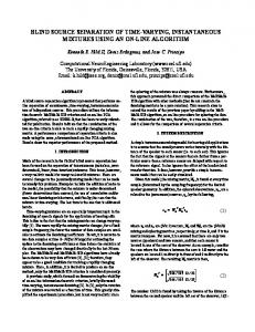
Figure 1.1: NMR spectra of two chemical compounds. In the circled region, βsitosterol (blue) has a stand-alone peak. Clearly, menthol (red) does not have such region. other words, each source signal must have a stand-alone peak where other sources are strictly zero there. Such a strict sparseness condition leads to a dramatic mathematical simplification of a general nonnegative matrix factorization problem (1.1) which is non-convex. Geometrically speaking, the problem of finding the mixing matrix A reduces to the identification of a minimal cone containing the columns of mixture matrix X. The latter can be done by linear programming. In fact, NN’s sparseness assumption and the geometric construction of columns of A were known in the 1990’s [2, 32] in the problem of blind hyper-spectral unmixing, where the same mathematical model (1.1) is used. The analogue of NN’s assumption is called pixel purity assumption [5]. The resulting geometric (cone) method is the so called N-findr [32], and is now a benchmark in hyperspectral unmixing. NN’s method can be viewed as an application of N-findr to NMR data. It is possible that measured NMR data may not strictly satisfy NN’s sparseness conditions, which introduces spurious peaks in the results. Postprocessing methods will be developed to address the resulting errors. Such a study has been performed recently in case of (over)-determined mixtures [29] where it is found that larger peaks in the signals are more reliable and can be used to minimize errors due to lack of strict sparseness. However, the geometric cone method (NN method, N-findr method) and its postprocessing would fail if the measured data do not satisfy NN assumption. Therefore, there is a need for new BSS methods which can separate non-NNA source signals. The following two examples show that a different condition on source signals is called for in this regard. Example 1: Consider the NMR spectra of two chemical compounds β-sitosterol and menthol in Fig. 1.1. As shown in the figure, β-sitosterol (blue) has standalone peaks however menthol (red) does not have such a peak. Hence NNA does not hold. Instead, β-sitosterol overlaps with menthol over the acquisition region and has dominant intervals over menthol in their NMR spectra.
2
Figure 1.2: Examples of standard NMR spectra of serum and urine, showing representative structural complexity produced by multiple metabolite signals (plot from [1]). Example 2: The data in Fig. 1.2 are from NMR spectroscopy of urine and blood serum. The complicated NMR spectra contain both wide-peak source signals and narrow-peak source signals. For example, the blood serum has constituents with wide spectral peaks which overlap others almost over the whole acquisition region. Similar signal peaks are observed in urine NMR spectrum. NN’s method and its postprocessing would not work for this type of data. The above two examples indicate that new BSS methods should be developed for these non-NNA signals. For the urine type NMR data, the method needs to be able to separate signals of wide spectral peaks from narrow peak signals. The method also should handle the signals with dominant intervals over one another, such as the data in example 1: though there are no wide peak signals, one source dominates the other over the region. In this paper, we shall develop a new BSS method to separate these two types of non-NNA data. This work is mainly motivated by NMR spectroscopy of urine and blood serum. Analysis of NMR spectra of biofluids such as urine and blood serum can provide extremely important information for metabolic fingerprinting and disease diagnosis (see [1, 31, 33, 34] and references therein). Identification and assignments of constituents in urine samples depends heavily on 2D NMR spectra. However, the complexity of urinary composition makes the complete assignments of the urinary spectra difficult, which is mainly due to the lack of reference spectra for unknown metabolites. Consequently, as of now, only about one-third of detectable urinary metabolites have been assigned unambiguously [34]. Similar situation exists in the NMR spectroscopy of blood serum. Our method can be used to separate and detect the unknown sources in the residuals of a regular spectra fitting with reference spectra data. In this context, it is unnecessary to separate all the source signals from urine and serum type data in a complete blind fashion. Our hope is to offer an assistive computational tool to produce a short list of possible unknown sources for a
3
knowledged chemist to pursue further analysis. The main challenge of the non-NNA problem we face is that the complicated NMR spectra contains both wide-peak source signals and narrow-peak source signals (in urine and serum NMR spectra). As a result, the mixing matrix A cannot be recovered from data matrix X independently of S as in [24], and so A and S are much more coupled. This paper uses divide and conquer strategy to retrieve A and S in a recursive way. The proposed method splits the source separation process into two major steps. The first step is a backward procedure where clustering and linear programming techniques are employed to recursively identify columns of the mixing matrix while simultaneously eliminating source variables. The first step also serves to convexify the orginal non-convex matrix factorization problem. Half of the unknowns are estimated. The second step is a forward step to solve a sequence of ℓ1 regularized convex optimization problems to recover the source signals. It should be pointed that although the method is motivated by the NMR spectroscopy of biofluids, the underlying ideas certainly can be generalized to other source separation applications. The paper is outlined as follows. In section 2, we propose a new condition on the source signals motivated by NMR spectroscopy data of biofluids. In section 3, we introduce our recursive BSS method. In section 4, we further illustrate our method with numerical examples including the processing of an experimental NMR data set. Section 5 is the conclusion. We shall use the following notations throughout the paper. The notation Aj stands for the j-th column of matrix A, S j for the j-th column of matrix S, X j the j-th column of matrix X. While Sj and Xj are the j-th rows of matrix S and X, or the j-th source and mixture, respectively. This work was partially supported by NSF-ADT grant DMS-0911277 and NSF grant DMS-0712881. The authors thank Professor A.J. Shaka and Dr. Hasan Celik for helpful discussions and their experimental NMR data.
2
Assumption on Source Signals
Let us consider the determined case (m = n). The results can be easily extended to over-determined case (m > n). Consider the linear model (1.1) where each column in X represents data collected at a particular value of the acquisition variable, and each row represents a mixture sprectrum. Recently the authors have developed a postprocessing approach on how to improve NN results with abundance of mixture data, and how to improve mixing matrix estimation with major peak based corrections [29]. The work in [29] actually considered a relaxed NNA (rNNA) condition Assumption (rNNA). : For each i ∈ {1, 2, . . . , n} there exists an ji ∈ {1, 2, . . . , p} such that si,ji > 0 and sk,ji = ǫk (k = 1, . . . , i − 1, i + 1, . . . , n) , where ǫk ≪ si,ji . Simply said, each source signal has a dominant peak at acquisition position where the other sources are allowed to be nonzero. NNA results if all ǫk = 0. The rNNA is more realistic and robust than the ideal NNA for real-world NMR data [24].
4
Motivated by the NMR spectra of urine and blood serum, we propose here a more general and relaxed condition on the source signals. Note that the rows S1 , S2 , . . . , Sn of S are the source signals, and they are required to satisfy the following condition: For i = 2, 3, . . . , n, source signal Si is allowed to have dominant interval(s) over Si−1 , . . . , S2 , S1 , while other part of Si may overlap with Si−1 , . . . , S2 , S1 . More formally, this condition implies that source matrix S satisfies the following condition Assumption. For each k ∈ {2, 3, . . . , n}, there is a set Ik ⊂ {1, 2, . . . , p} such that for each l ∈ Ik sil ≫ sjl , i = k, k + 1, . . . , n, j = 1, 2, . . . , k − 1. We shall call this dominant interval condition, or DI condition. In simple terms, the condition DI requires dominant interval(s) from each source signal over some of the other source signals in a hierarchical manner. Fig. 3.1 is an idealized example of three DI source signals. For the application of NMR spectroscopy of urine and serum that motivated us, the DI source conditions hold well.
3
The Method
In this section, we introduce a recursive BSS method to separate the DI source signals. For the purpose of illustration, we shall use the simulated data (Fig. 3.1 – Fig. 3.6, Fig. 4.1– Fig. 4.8) for which we did not specify units. But the unit of the x-axis can be understood as number of pixels. A real NMR spectrum usually has ppm (parts per million) as its unit (see the real data in Fig. 4.9–Fig. 4.11). The method consists of two main steps: forward step and backward step. It starts with the backward step where the BSS problem is reduced to a series of sub-BSS problems.
3.1
Backward step: model reduction
Consider to separate n DI sources from n mixtures. Condition DI implies that there is region where source Sn dominates others. More precisely, there are columns of X such that n−1 X k n X = sn,k A + oi,k Ai , (3.1) i=1
where sn,k dominate oi,k (i = 1, . . . , n − 1), i.e., sn,k ≫ oi,k . The identification of An is equivalent to finding a cluster formed by these X k ’s in Rn . As illustrated in Fig. 3.1, source signal S3 has two dominant peak regions R1 , R2 which satisfy (3.1), hence a cluster is formed in Fig. 3.1. Next we shall discuss how to locate the cluster (thus An ). All X’s column vectors form a set of points P = {X 1 , X 2 , . . . , X p } in n dimensional space. The convex hull of P is a polytope, A in Rn . The frame F of these points is the set of extreme points of the convex hull. To determine if the element X k of the set P constitutes an element of F , the following constrained problem is suggested p X
X j λj = X k ,
λj ≥ 0,
k = 1, . . . , p.
(3.2)
j=1,j6=k
X k belongs to F if it cannot be written as a linear combination of other points of P. Linear programming can be used to solve (3.2). Apparently, F contains a vector 5
1.5
S
1
1 0.5 0
0.34 0
20
40
60
80
100
120
140
160
180
200
0.32
1.5
S R3
0.5 0
0.3
2
1
0.28
0.26 0
20
40
60
80
100
120
140
160
180
200
0.24 0.4
1.5 R1
R2
S
3
1
0.38 0.36
0.5 0
0.34 0.32 0
20
40
60
80
100
120
140
160
180
200
0.3
0.345
0.35
0.355
0.36
0.365
0.37
0.375
0.38
0.385
0.39
0.395
Figure 3.1: Left plot is the three DI source signals, notice that S3 has two dominant regions R1 and R2 over S2 and S1 , while S2 dominates S1 in region R3 . Recognizing each of column vectors of the mixture matrix X as a point in 3D space, we show the geometry of X in the second plot, the convex hull of X consists of eight points, the one attracting a cluster is recognized as A3 . which is approximately parallel to An , this can be seen from equation (3.1). Among the elements of F , An is the one attracting a cluster. To identify An , an ǫ-ball is created with center at each element of F . The center of the ball that contains most of data points is recognized as An . After An is obtained, we reduce the model by eliminating Sn from X. Denoting the n mixtures as row vectors X1 , . . . , Xn , let us write (1.1) as hP i Pn−1 Pn−1 n−1 X1 = j=1 A1j Sj1 + A1n Sn1 , j=1 A1j Sj2 + A1n Sn2 , . . . , j=1 A1j Sjp + A1n Snp hP i Pn−1 Pn−1 n−1 A S + A S , A S + A S , . . . , A S + A S X2 = 2j j1 2n n1 2j j2 2n n2 2j jp 2n np j=1 j=1 j=1
.. .
Xn =
hP n−1 j=1
Anj Sj1 + Ann Sn1 ,
Pn−1 j=1
Anj Sj2 + Ann Sn2 , . . . ,
Pn−1 j=1
Anj Sjp + Ann Snp
(3.3) where A = [A1n , A2n , . . . , Ann ] is already retrieved from the data clustering. Using in Xn , the last equation of (3.3), we eliminate Sn by the transformation Xi → Xi − AAnn i = 1, 2, . . . , n − 1. Then a new mixture matrix is formed as 1n X1 − AAnn Xn X2 − A2n Xn Ann X(1,2,...,n−1) = (3.4) ∈ R(n−1)×p .. . n
T
Xn−1 −
An−1,n Xn Ann
which contains n − 1 mixtures from source signals S1 , . . . , Sn−1. In fact, we formulate 6
i
The convex hull 1
12 10
0.9
8 6
0.8
4
0.7
2 0
0
20
40
60
80
100
120
0.6
140
0.5
4
0.4
3
2
0.3
1
0.2
0
0
20
40
60
80
100
120
0.1
140
0.4
0.5
0.6
0.7
0.8
0.9
1
Figure 3.2: Left is the two mixtures after eliminating the third source, their geometric plot is on the right. From the picture, the mixing coefficients of the second source in the mixtures attracts a cluster of points (red circle). a reduced BSS model e(1,2,...,n−1) S(1,2,...,n−1) , X(1,2,...,n−1) = A
e(1,2,...,n−1) is the mixing matrix of the source S1 , . . . , Sn−1 in the reduced mixwhere A tures X(1,2,...,n−1) . In the new mixtures X(1,2,...,n−1) , source Sn−1 has dominant regions over other sources. Therefore, the data clustering and linear programming can be used to recover the mixing coefficients of Sn−1 from X(1,2,...,n−1) . Then we reduce the mixtures further to X(1,2,...,n−2) containing S1 , . . . , Sn−2 . For example, Fig. 3.2 shows the two resulting mixtures after eliminating S3 from the three mixtures in Fig. 3.1. For k ≤ n − 1, data clustering, linear programming combined with mixtures reduction will be recursively employed until source S1 is obtained. The following intermediate reduced mixtures are produced during the recursive process e(1,2,...,k) S(1,2,...,k) X(1,2,...,k) = A
for k = 1, 2 . . . , n − 1 ,
(3.5)
e(1,2,...,k) is the mixing matrix of the source S1 , . . . , Sk in the reduced mixtures where A X(1,2,...,k). In summary, the backward step not only extracts source signal S1 , but also generates a series of reduced mixtures X(1,2) , X(1,2,3) , . . . , X(1,2,...,k) , . . . , X(1,2,...,n−1) . It should be noted that although the original BSS model (1.1) contains nonnegative A, S and X, the reduced mixtures and mixing matrices may have negative entries from the variable eliminations, meaning that the intermediate mixtures allows general linear combinations of the nonnegative source signals. The geometric cone method is still able to identify the minimal cone which contains the columns of X(1,2,...,k) , k = 2, . . . , n − 1, only that the cone may not lie in the sector consisting of nonnegative vectors.
3.2
Forward step: recovery of the sources
With S1 being recovered, we shall discuss how to separate the source signals S2 , . . . , Sn . It can be verified in that the solution of Sk , k = 2, . . . , n is not unique given its mixing 7
coefficients in mixture X(1,2,...,k) and S1 , S2 , . . . , Sk−1. In fact, if we consider to solve e(1,2) S1,2 in terms of components for S2 , then we write X1,2 = A � � � � � � x11 x12 · · · x1p a11 a12 s11 s12 · · · s1p = · , x21 x22 · · · x2p a21 a22 s21 s22 · · · s2p where the known components are denoted in color black, while the unknown variables are in color red. To solve the unknown aij ’s (there are 2 in this case), we select the first two columns of X to set up the following four equations: x11 = a11 s11 + a12 s21 x =a s +a s 12 11 12 12 22 x21 = a21 s11 + a22 s21 x22 = a21 s12 + a22 s22 and they can be written in matrix form Q Y = b s11 0 a12 s12 0 0 Q= 0 s11 a22 0 s12 0
with 0 a12 , 0 a22
Y = (a11 , a21 , s21 , s22 )T , b = (x11 , x12 , x21 , x22 )T . In fact, performing column addition operations on Q by a12 to eliminate s11 and s12 in the top left corner, we obtain 0 0 a12 0 0 0 a12 a220 − a s11 s11 a22 0 , 12 − aa22 s12 s12 0 a22 12 then the first column can be eliminated by the second column. Therefore matrix Q is singular, which implies that S2 does not have unique solutions even up to scaling. It can be deduced that S3 , . . . , Sn are non-unique by similar arguments. It appears that solving the equation exactly for S2 , . . . , Sn is hopeless However a meaningful solution is possible if the actual source signals are structurally compressible, meaning that they essentially depend on a low number of degrees of freedom. For instance, if our source signal is sparse in some transformed domain, then the problem is readily simplified, and the search for solutions becomes feasible. According to analytical chemistry [12], an NMR spectrum is represented as a sum of symmetrical, positive valued, Lorentzian-shaped peaks. Therefore, the NMR spectrum can be thought as a linear convolution of Lorentzian kernel with some sparse function consisting of few sharp peaks, or more precisely, S = Sˆ ∗ L(x, w) , 1 w 1 2 where L(x, w) = , w specifies its width (full width at half maximum), π x2 + ( 21 w)2 and Sˆ is a sparse function. In Fig. 3.3, the NMR signal (dashdot line) is a convolution
8
3
2.5
2
1.5
1
0.5
0
0
20
40
60
80
100
120
140
Figure 3.3: NMR signal (dashdot line) is a convolution of a sparse signal (solid line) with a Lorentzian kernel of width = 4. of a sparse (solid line) with Lorentzian kernel of width = 4. The sparsity under the Lorentzian kernel suggests that an ℓ1 minimization problem can be formulated to recover the source signals. For example, consider the recovery of S2 . Recall that source S1 is recovered and the reduced mixture matrix X(1,2) is generated in the backward step. The fact that source S1 is sparse under the Lorentzian kernel and that mixture signals may in general contain noise suggest solving the following optimization problem: min
A(1) ∈R2×1 , 2×p , S≥0 ˆ ˆ S∈R
ˆ 1 + 1 kX(1,2) − A(1) S1 − Sˆ ∗ L(w2)k2 , µkSk 2 2
(3.6)
where X(1,2) ∈ R2×p is a mixture matrix containing source S1 and S2 , p is the number of available samples. A(1) is a column vector containing the mixing coefficients of source S1 in X(1,2) . Each row of Sˆ stands for a sparse function with few sharp peaks, and the rows of Sˆ ∗ L(w2 ) are the multiples of source S2 in X(1,2) . The linear convolution Sˆ ∗ L is approximated by a matrix multiplication Sˆ L in the computation, here L ∈ Rp×p is the discretized Lorentzian kernel. w2 is the peak width of S2 , the estimation of this parameter will be discussed later. In general, to recover Sk for k = 2, . . . , n−1, the following ℓ1 minimization problem is proposed: min
A(1,2...,k−1) ∈Rk×(k−1) , k×p , S≥0 ˆ ˆ S∈R
ˆ 1 + 1 kX(1,2,...,k) − A(1,2...,k−1) S(1,2,...,k−1) − Sˆ ∗ L(wk )k2 , (3.7) µkSk 2 2
where X(1,2,...,k) ∈ Rk×p is the mixture matrix which contains sources S1 , . . . , Sk , the columns of A(1,2...,k−1) ∈ Rk×(k−1) correspond to the mixing coefficients of source S1 , . . . , Sk−1 in X(1,2,...,k) , respectively. The rows of Sˆ ∗ L(wk ) represent multiples od source Sk in X(1,2,...,k) , wk is the peak width of Sk . Because (3.7) allows the constraint A(1,2...,k−1) S(1,2,...,k−1) + Sˆ ∗L(wk ) = X(1,2,...,k) to be relaxed, it is applicable when 9
the mixtures are contaminated by measurement errors such as instrument noise. The l2 norm in (3.7) is to model the unknown measurement error or noise as Gaussian. When there is minimal measurement error, one must assign a tiny value to µ to heavily weigh the fidelity term kX(1,2,...,k) − A(1,2...,k−1) S(1,2,...,k−1) − Sˆ ∗ L(wk )k22 in order for A(1,2...,k−1) S(1,2,...,k−1) + Sˆ ∗ L(wk ) = X(1,2,...,k) to be nearly satisfied. In this case, one could also formulate an optimization problem as: ˆ 1 , s.t. A(1,2...,k−1) S(1,2,...,k−1) + Sˆ ∗ L(wk ) = X(1,2,...,k) , Sˆ ≥ 0, min kSk
(3.8)
for which Bregman iterative method [14, 35] with a proper projection onto nonnegative convex subset can be used to obtain a solution. The equality constraint of (3.8) contains k × p number of equations and k × (k − 1 + p) variables, which implies that it is under-determined. When measurement noise is minimal, the region defined by the equality and inequality constraints is non-empty. For simplicity, we solve (3.7) by the projected gradient descent (PGD) approach. The following multiplicative update rules preserve the nonnegativity constraints for ˆ nonnegative initial data for S: aij ← aij � sˆjk
�
T T X S(1,2,...,k−1) − Sˆ L S(1,2,...,k−1)
A(1,2,...,k−1) S
�
ij � , T (1,2,...,k−1) S(1,2,...,k−1) ij
h� i � (1,2,...,k−1) XL−A S(1,2,...,k−1) L jk − µ + ← sˆjk , � � ˆ S L L jk
(3.9)
(3.10)
ˆ jk . For where the nonlinear operator [x]+ = max{0, x}, aij = (A(1,2,...,k−1) )ij , sˆjk = (S) the convex objective (3.7), the iterations in (3.9)-(3.10) converge to a global minimum. At this point, we have retrieved S1 , . . . , Sn−1 . Next, we separate the last source signal Sn from the original mixtures matrix X. We consider to solve the following ℓ1 minimization problem, min
0≤A(1,...,n−1) ∈Rn×(n−1) , , n×p , S≥0 ˆ ˆ S∈R
ˆ 1 + 1 kX − A(1,...,n−1) S(1,...,n−1) − Sˆ ∗ L(wn )k2 , µkSk 2 2
(3.11)
Where rows of X ∈ Rn×p represent the n mixture signals, the columns of A(1,...,n−1) correspond to the mixing coefficients of S1 , . . . , Sn−1 in X. The rows of Sˆ ∗ L(wn ) are the multiples of Sn in X. Again, we use gradient descent approach to solve (3.11). The following multiplicative update rules are applied h� � i T T ˆ X S(1,2,...,n−1) − S L S(1,2,...,n−1) ij � +, aij ← aij � (1,2,...,n−1) T A S(1,2,...,n−1) S(1,2,...,k−1) ij sˆjk ← sˆjk
h�
i � X L − A(1,2,...,k−1) S(1,2,...,k−1) L jk − µ + , � � ˆ S L L jk
ˆ jk . This problem is similar to (3.7). The difwhere aij = (A(1,2,...,n−1) )ij , sˆjk = (S) ference is that, in (3.7) the nonnegativity constraint is only imposed to the source 10
120
100
80
60
40
20
0
0
100
200
300
400
500
600
Figure 3.4: A second order Butterworth low pass filter is designed to estimate the peak width of wide peak signal. The solid curve is the mixture signal, the dashed curve is the filtered wide peak signal from which an estimation of peak width can be read off. signals, while in (3.11) both the mixing matrix and sources are required to be nonnegative. As explained in section 3.1, the intermediate mixtures X(1,2) , . . . , X(1,2,...,n−1) could have negative entries from the variables elimination, meaning that subtractive combinations of nonnegative sources could exist in these mixtures. For the peak width parameter used in the ℓ1 computations, estimate of an upper bound suffices. A straightforward way is to read off approximate value from mixture signals if the dominant interval(s) happen to contain a peak. For more complicated mixture signals, a low pass filter could be designed to extract more accurate estimation (see Fig. 3.4). In the practice of NMR, the expertise of an analytical chemist may also be helpful to estimate this parameter. The PGD approach is sufficient for examples we studied here, however Bregman method might be more suitable for solving larger size problems due to its efficiency. We shall make a comparison between the Bregman iterative method and the PGD approach used in the paper in terms of time cost and convergence. We use the linearized Bregman method [14, 35] to solve (3.8). We consider to solve the related unconstrained minimization problem (3.7). Rewrite the problem with new notations as follows ˆ 1 + 1 kf T − M W − Sˆ Lk2 , min µkSk (3.12) 2 2 M ∈Rk×(k−1) , k×p , S≥0 ˆ ˆ S∈R
T where M = A(1,2...,k−1) ∈ Rk×(k−1) , f = X(1,2,...,k) ∈ Rp×k , W = S(1,2,...,k−1) ∈ R(k−1)×p . � T � � � M Let us introduce u = ∈ R(k−1+p)×k , B = W T , L ∈ Rp×(k−1+p) , then (3.12) T ˆ S reads 1 min µkP uk1 + kBu − f k22 , (3.13) 2
11
4
3
10000
x 10
source 1
2 5000
1 0
0
200
400
600
800
1000
1200
1400
1600
0
1800
0
200
400
600
800
1000
1200
1400
1600
1800
10000
15000
source 2
10000
5000 5000 0
0
200
400
600
800
1000
1200
1400
1600
0
1800
0
200
400
600
800
1000
1200
1400
1600
1800
15000
10000
source 3
10000 5000
5000 0
0
200
400
600
800
1000
1200
1400
1600
0
1800
0
200
400
600
800
1000
1200
1400
1600
1800
Figure 3.5: three mixtures (left column), and the sources (right column). �
� O(k−1)×k where P = . The linearized Bregman method can be written iteratively Ip×k by introducing an auxiliary variable v j : j+1 j − B T (B uj − f ), v j+1 = v j+1 ui = vi , for i = 1, . . . , k − 1, (3.14) � j+1 j+1 u = δ · shrink+ (v , µ , for i = k, . . . , k − 1 + p, i
i
where u0 = v 0 = O, δ > 0 is the step size, and shrink+ is for computing nonnegative solutions, � � v − µ, if v > µ, shrink+ (v, µ = (3.15) 0, if v < µ,
Note that the first k − 1 rows from v j are assigned to M T which is (A(1,2,...,k))T , and the rest rows are given to SˆT . The synthetic data used for testing the two methods is three mixtures from three sources shown in Fig. 3.5. Suppose source 1 and 2 have been recovered, source 3 will be solved by (3.7) using (3.9)-(3.10) and linearized Bregman iteration. Computation is performed on a Dell laptop with 6G RAM and 1.6 GHz i7 CPU. The results are shown in Fig. 3.6. The cpu time for the top-left plot (PGD approach) is 7.98 seconds, and it is 3.92 seconds for the top-right plot (linearized Bregman). It can be seen that Bregman iteration converges faster than the PGD approach. We remark that although our recursive BSS framework is motivated by the NMR spectroscopy of biofluids, the idea can be applied to separating other NMR data. In practice, we might only need to perform the backward and forward steps once instead of recursively. In the next section, we shall process an expermental data set. We shall use clustering to retrieve all the columns of the mixing matrix, then retrieve the sources by solving a nonnegative ℓ1 optimization problem. The elimination of variables (model reduction) is unnecessary for this example. 12
0.7
0.7
0.6
0.6
0.5
0.5
0.4
0.4
0.3
0.3
0.2
0.2
0.1
0.1
0
0
200
400
600
800
1000
1200
1400
1600
0
1800
0
200
400
600
800
1000
1200
1400
1600
1800
−3
12
x 10
PGD linearized Bregman 10
Error
8
6
4
2
0 10
20
30
40
50
60
70
80
number of iterations
Figure 3.6: results by PGD approach (top-left), and linearized Bregman iteration (top-right), and the convergence of the methods (bottom column).
13
4
Numerical Computations
In this section, we report the numerical examples solved by the method. We compute three examples. The data of the first two examples are synthetic. In the first example, three sources are to be separated from three mixtures, one source is supposed to have narrow peaks, one has relatively wide peaks, and the last one has very wide peaks. The results are presented in a series of plots. Fig. 4.1 to Fig. 4.3 illustrate the backward step, and Fig. 4.4 presents the recovered source signals by ℓ1 minimization in the forward step. In the step of recovering the source signal S2 and S3 via ℓ1 minimization, the peak widths w2 = 60, w3 = 130 are read off from the mixture signals. Compared to ground truth, the separation results by our method are accurate. In the second example, we used true NMR spectra of menthol and β-sitosterol (see their reference spectra in Fig. 4.6) as sources. The mixtures are created following model (1.1). We also added gaussian noise to the data to test the robustness of the method. The two mixtures are plotted in Fig. 4.5. The computed results by the method are shown in Fig. 4.7- Fig. 4.8. Comparing the two calculated spectra of β-sitosterol in Fig. 4.8, ℓ1 minimization generates a sparser solution and proves to be robust to noise. For the third example, we provide a set of real data to test our method. The data is produced by diffusion ordered spectroscopy (DOSY) which is an NMR spectroscopy technique used by chemists for mixture separation [21]. However, the three compounds used in the experiment (quinine, geraniol, and camphor) have similar chemical functional groups (i.e. there is overlap in their NMR spectra) [23], for which DOSY fails to separate them. Though our working hypothesis is not satisfied completely, it is known that each of the three sources has dominant interval(s) over others in its NMR spectrum. This can also be verified from the three isolated clusters formed in their mixed NMR spectra (see the geometry of their mixtures in Fig. 4.9). Here we separate three sources from three mixtures. Fig. 4.9 plots the mixtures (rows of X) and their geometry (columns of X) where three clusters of points can be spotted. Then the columns of A are identified as the center points of three clusters. Note that elimination of variables is not necessary since all A’s columns have been obtained by one time clustering (K-means). The three isolated clusters imply that the source matrix S possesses column sparsity, therefore we consider to solve the following nonnegative ℓ1 optimization (for each column S i of S): min kS i k1
subject to AS i = X i , for i = 1, . . . , p
(4.1)
for the recovery of the sources S. Problem (4.1) is a linear program because S i is non-negative, also solvable by PGD approach and Bregman iterative method. The solutions are presented in Fig. 4.10, the results are satisfactory comparing with the ground truth. As a comparison, the source signals recovered by NN [24] is shown in Fig. 4.11 where S = inverse(A) X, here the inverse is Moore-Penrose (least square sense) pseudo-inverse which produces some negative (erroneous) peaks in S.
5
Conclusion
This paper presented a novel BSS method for nonnegative and correlated data. The motivation lies in the NMR spectroscopy of urine and serum for metabolic fingerprinting and disease diagnosis. Inspired by the NMR structure of urine type data, we 14
150 0.31 100 0.3 50 0
0.29 0
100
200
300
400
500
600
700 0.28
100
0.27 50 0.26 0
0
100
200
300
400
500
600
700
0.25
100 0.24 50
0
0.23
0.22 0
100
200
300
400
500
600
700 0.3
0.305
0.31
0.315
0.32
0.325
0.4 0.3350.35
0.33
0.45
Figure 4.1: Backward step 1, On the left: the three mixtures; On the right: the geometry of the mixture and the recovery of A3 (the one in the blue circle). From the plots of the mixtures, there is dominant region containing a spectral peak (in the red rectangle), hence an estimation w3 = 130 for the peak width of source S3 can be read off.
50
0.4
40
0.38
30 0.36 20 0.34 10 0
0.32 0
100
200
300
400
500
600
700 0.3
10
0.28
8 0.26 6 0.24 4 0.22
2 0
0
100
200
300
400
500
600
0.2 0.91
700
0.92
0.93
0.94
0.95
0.96
0.97
0.98
Figure 4.2: Backward step 2. Model reduction via eliminating S3 . The plots are the two mixtures and their geometry. It can be seen from the plot the mixing coefficients of source S2 in X(1,2) attracts a cluster of points. An estimation of w2 = 60 (peak width of S2 ) is read off from peaks in the rectangular region.
15
18 16 14 12 10 8 6 4 2 0 −2
0
100
200
300
400
500
600
700
Figure 4.3: Backward step 3. The recovery of S1 by eliminating S2 from the reduced mixture X(1,2) .
4
6
2
4
0
2
−2
0
100
200
300
400
500
600
0
700
8
4
6
3
4
2
2
1
0
0
100
200
300
400
500
600
0
700
40
8
30
6
20
4
10
2
0
0
100
200
300
400
500
600
0
700
0
100
200
300
400
500
600
700
0
100
200
300
400
500
600
700
0
100
200
300
400
500
600
700
Figure 4.4: Forward step. Left is the recovered sources by ℓ1 minimization. Right is the reference spectra.
16
6 5 4 3 2 1 0 −1
0
100
200
300
400
500
600
700
800
900
0
100
200
300
400
500
600
700
800
900
3 2.5 2 1.5 1 0.5 0 −0.5
Figure 4.5: Spectra of two mixture samples of menthol and β-sitosterol. propose a working hypothesis which requires dominant interval(s) from each source signal over some of the other source signals in a hierarchical manner. The hierarchy form of the dominant interval(s) enables the development of a novel BSS method which recursively breaks the BSS problem down into a series of sub-BSS problems by a combination of data clustering, linear programming, and variables elimination. From the intermediate sub-BSS problems, the source signals are retrieved by repeatedly solving an ℓ1 minimization problem in a sparse transformed domain. Numerical results on NMR spectra data show satisfactory performance of our method and offer promise towards understanding and detecting complex chemical spectra for health sciences.
References [1] R. Barton, J. Nicholson, P. Elliot, and E. Holmes, High-throughput 1H NMR-based metabolic analysis of human serum and urine for large-scale epidemiological studies: validation study, Int. J. Epidemiol. 37(2008)(suppl 1)pp. i31–i40. [2] J. Boardman, Automated spectral unmixing of AVRIS data using convex geometry concepts, in Summaries of the IV Annual JPL Airborne Geoscience Workshop, JPL Pub. 93-26, Vol. 1, 1993, pp 11-14. [3] P. Boflla and M. Zibulevsky, Underdetermined blind source separation using sparse representations, Signal Processing, 81 (2001) pp. 2353–2362. [4] J. Cai, S. Osher, and Z. Shen, Linearized Bregman iterations for compressed sensing, UCLA CAM Report, vol. 08, no. 06, 2008. [5] C-I Chang, ed., “Hyperspectral Data Exploitation: Theory and Applications”, Wiley-Interscience, 2007. 17
0.3 0.25 0.2 0.15 0.1 0.05 0
0
100
200
300
400
500
600
700
800
900
0
100
200
300
400
500
600
700
800
900
0.6 0.5 0.4 0.3 0.2 0.1 0
Figure 4.6: Reference spectra of β-sitosterol and menthol.
18
2.5
2
1.5
1
0.5
0
−0.5
0
100
200
300
400
500
600
700
800
900
Figure 4.7: Computed source spectrum of menthol. [6] S. Choi, A. Cichocki, H. Park, and S. Lee, Blind source separation and independent component analysis: A review, Neural Inform. Process. Lett. Rev., 6 (2005), pp. 1–57. [7] A. Cichocki and S. Amari, Adaptive Blind Signal and Image Processing: Learning Algorithms and Applications, John Wiley and Sons, New York, 2005. [8] P. Comon, Independent component analysis–a new concept?, Signal Processing, 36 (1994) pp. 287–314. [9] P. Comon and C. Jutten, Handbook of Blind Source Separation: Independent Component Analysis and Applications, Academic Press, 2010. [10] D. Donoho and J. Tanner, Sparse nonnegative solutions of underdetermined linear equations by linear programming, Proc Natl Acad Sci USA, 102 (2005) pp. 9446?9451. [11] I. Drori, Fast ℓ1 minimization by iterative thresholding for multidimensional NMR spectroscopy, EURASIP Journal on Advances in Signal Processing, 2007, No. 23, pp 1-10 (doi:10.1155/2007/20248). [12] R. Ernst, G. Bodenhausen, and A. Wokaun, Principles of Nuclear Magnetic Resonance in One and Two Dimensions, Oxford University Press, 1987. [13] P. Georgiev, F. Theis, and A. Cichocki, Sparse component analysis and blind source separation of underdetermined mixtures, IEEE Transactions on Neural Networks, 16(4) (2005) pp. 992–996. [14] Z. Guo and S. Osher, Template matching via ℓ1 minimization and its application to hyperspectral target detection, Tech. Rep. 09-103, UCLA, www.math.ucla.edu/applied/cam/, 2009. 19
1.8
1.6
1.4
1.2
1
0.8
0.6
0.4
0.2
0
0
100
200
300
400
500
600
700
800
900
0
100
200
300
400
500
600
700
800
900
1.8
1.6
1.4
1.2
1
0.8
0.6
0.4
0.2
0
Figure 4.8: Computed source spectrum of β-sitosterol by ℓ1 minimization using different µ values. Top: µ = 0. Bottom: µ = 0.09. The ℓ1 penalty provides a sparser solution in the bottom panel.
20
4
10
x 10
5
0 10
9
8
7
6
5
4
3
2
1
0
9
8
7
6
5
4
3
2
1
0
9
8
7
6
5
4
3
2
1
0
4
6 0.14
x 10
4
0.12 2 0.1 0.34
0.08
0 10
0.345
0.06 0.6
15000
0.35 0.58 0.355
0.56 0.54
10000
0.36 0.52
5000
0.365
0.5 0.48
0 10
0.37
ppm
Figure 4.9: three columns of A are identified as the three center points in blue circles attracting most points in scatter plots of the columns of X (left), and the three rows of X (right).
4
15
x 10
geraniol
10000 10 5000 5 0 10
9
8
7
6
5
4
3
2
1
0 10
0
9
8
7
6
5
4
3
2
1
0
4
3
2
1
0
4
3
2
1
0
4
6
x 10
quinine
10000 4 5000 2 0 10
9
8
7
6
5
4
3
2
1
0 10
0
9
8
7
6
5
4
10
x 10
camphor
10000 5
0 10
5000
9
8
7
6
5
4
3
2
1
0 10
0
9
8
7
6
5
ppm
ppm
Figure 4.10: the recovered source signals by nonnegative ℓ1 (left) and the ground truth (right).
21
30
geraniol
10000
20 10
5000
0 −10 10
9
8
7
6
5
4
3
2
1
0 10
0
9
8
7
6
5
4
3
2
1
0
4
3
2
1
0
4
3
2
1
0
10
quinine
10000 5 5000
0 −5 10
9
8
7
6
5
4
3
2
1
0 10
0
9
8
7
6
5
10
camphor
10000 5 5000
0 −5 10
9
8
7
6
5
4
3
2
1
0 10
0
ppm
9
8
7
6
5
ppm
Figure 4.11: the recovered source signals using NN method (left) and the ground truth (right). [15] A. Hyv¨arinen, J. Karhunen and E. Oja, Independent Component Analysis, John Wiley and Sons, New York, 2001. [16] I. Koprivaa, I. Jeri´c, and V. Smreˇcki, Extraction of multiple pure component 1H and 13C NMR spectra from two mixtures: Novel solution obtained by sparse component analysis-based blind decomposition, Analytica Chimica Acta, 653 (2009) pp. 143–153. [17] D. D. Lee and H. S. Seung, Learning of the parts of objects by non-negative matrix factorization, Nature, 401 (1999) pp. 788–791. [18] J. Liu, J. Xin, Y-Y Qi, A Dynamic Algorithm for Blind Separation of Convolutive Sound Mixtures, Neurocomputing, 72(2008), pp 521-532. [19] J. Liu, J. Xin, Y-Y Qi, A Soft-Constrained Dynamic Iterative Method of Blind Source Separation, SIAM J. Multiscale Modeling Simulations, Vol. 7, No. 4, pp 1795-1810, 2009. [20] J. Liu, J. Xin, Y-Y Qi, F-G Zeng, A Time Domain Algorithm for Blind Separation of Convolutive Sound Mixtures and L-1 Constrained Minimization of Cross Correlations, Comm. Math Sci, Vol. 7, No. 1, 2009, pp 109-128. [21] G. Morris, In Encyclopedia of Nuclear Magnetic Resonance, D. Grant, R. Harris, Eds, John Wiley & Sons, 2002. [22] S. Moussaouia, H. Hauksd´ottir, F. Schmidt, C. Jutten, J. Chanussot, D. Briee, S. Dout´e, and J.A. Benediktsson, On the decomposition of Mars hyperspectral data by ICA and Bayesian positive source separation, Neurocomputing, 71(2008), pp 2194–2208.
22
[23] M. Nilsson, M. Connel, A. Davies, and G. Morris, Biexponential Fitting of Diffusion-Ordered NMR Data: Practicalities and Limitations, Analytical Chemistry, 78 (2006), pp. 3040–3045. [24] W. Naanaa and J.–M. Nuzillard, Blind source separation of positive and partially correlated data, Signal Processing 85 (9) (2005), pp. 1711–1722. [25] D. Nuzillard, S. Bourgb and J.–M. Nuzillard, Model-Free analysis of mixtures by NMR using blind source separation, J. Magn. Reson. 133 (1998) pp. 358–363. [26] M. Plumbley, Conditions for non-negative independent component analysis, IEEE Signal Processing Letters, 9 (2002) pp. 177–180. [27] M. Plumbley, Algorithms for nonnegative independent component analysis, IEEE Transactions on Neural Networks, 4(3) (2003) pp. 534–543. [28] K. Stadlthanner, A. Tom, F. Theis, W. Gronwald, H.-R. Kalbitzer, and E. Lang, On the use of independent analysis to remove water artifacts of 2D NMR Protein Spectra, In Proc. Bioeng’2003 (2003). [29] Y. Sun, C. Ridge, F. del Rio, A.J. Shaka and J. Xin, Postprocessing and Sparse Blind Source Separation of Positive and Partially Overlapped Data, Signal Processing 91 (2011) pp. 1838–1851 [30] Y. Sun and J. Xin,Unique Solvability of Under-Determined Sparse Blind Source Separation of Nonnegative and Partially Overlapped Data, IASTED International Conference on Signal and Image Processing, 710-017, August 23–25, 2010, Hawaii, USA. [31] C. Vitols and A. Weljie, Identifying and Quantifying Metabolites in Blood Serum and Plasma, Chenomx Inc., 2006. [32] M.E. Winter, N-findr: an algorithm for fast autonomous spectral endmember determination in hyperspectral data, in Proc. of the SPIE, vol. 3753, 1999, pp 266-275. [33] W. Wu, M. Daszykowski, B. Walczak, B.C. Sweatman, S. Connor, J. Haselden, D. Crowther, R. Gill, M. Lutz, Peak alignment of urine NMR spectra using fuzzy warping, J. Chem. Inf. Model., 46(2006) pp. 863–875. [34] W. Yang, Y. Wang, Q. Zhou, and H. Tang, Analysis of human urine metabolites using SPE and NMR spectroscopy, Sci China Ser B-Chem, 51(2008) pp. 218–225. [35] W. Yin, S. Osher, D. Goldfarb, J. Darbon, Bregman iterative algorithm for ℓ1 -minimization with applications to compressive sensing, SIAM J. Image Sci, 1(143), pp 143-168, 2008.
23