three types of algorithms for blind source separation (BSS) of a convolutive ..... measure the cross talk powers before and after separation. The second fteen ...
1
On-line Blind Source Separation of Non-Stationary Signals
Lucas Parra, Clay Spence Sarno� Corporation, CN-5300, Princeton, NJ 08543, lparra@sarno�.com, cspence@sarno�.com Abstract | We have shown previously that non-stationary signals recorded in a static multi-path environment can often be recovered by simultaneously decorrelating varying second order statistics. As typical sources are often moving, however, the multi-path channel is not static. We present here an on-line gradient algorithm with adaptive step size in the frequency domain based on second derivatives, which we refer to as multiple adaptive decorrelation (MAD ). We compared the separation performance of the proposed algorithm to its o�-line counterpart and to another decorrelation based on-line algorithm.
I. Introduction
Blind source separation is an ongoing research topic. Among the unresolved problems we consider two of particular importance. First, most of the known algorithms try to invert a multi-path acoustic environment by nding a multi-path nite impulse response (FIR) lter that approximately inverts the forward channel. However, a perfect inversion may require fairly long FIR lters. In our experience such situations occur in strongly echoic and reverberant rooms where most, if not all, current algorithms fail. Secondly, changing forward channels due to moving sources, moving sensors, or changing environments require an algorithm that converges su�ciently quickly to maintain an accurate current inverse of the channel. It is this second problem that we address here. In terms of separation criteria to our knowledge there are three types of algorithms for blind source separation (BSS ) of a convolutive mixture of broad-band signals. Algorithms that diagonalize a single estimate of the second order statistics, algorithms that simultaneously diagonalize second order statistics at multiple times exploiting non-stationarity, and algorithms that identify statistically independent signals by considering higher order statistics. The simpler algorithms generate decorrelated signals by diagonalizing second order statistics [1], [2]. They have a simple structure that can be implemented e�ciently[1], [3], [4], but are not guaranteed to converge to the right solution as single decorrelation is not a su�cient condition to obtain independent model sources [5], [1], [2]. Instead, for stationary signals higher order statistics have to be considered [6], either by direct measurement and optimization of higher order statistics [6], [7], [8], [9], [10], or indirectly by making assumptions on the shape of the cumulative denSubmitted to VLSI Signal Processing Systems, March 25, 1999. Accepted December 16, 1999. To be published in special issue on 1998 IEEE Neural Networks and Signal Processing Workshop. Expected for summer 2000.
sity function (cdf ) of the signals [11], [12], [13]. The former methods are fairly complex and di�cult to implement. The latter methods fail in cases where the assumptions on the cdf are not accurate. Finally, for non-stationary signals it is known [1], and has been demonstrated [14], [15], [16], [17], that one may recover the signals by simultaneously diagonalizing second order statistics estimated at di�erent times. On-line algorithms are available for the single decorrelation [1], [2], [3], [18] approach and the indirect higher order methods [19], [20], but they have the same limitations as their o�-line counterparts. More recently a number of single decorrelation algorithms have been presented that claim good performance for non-stationary signals. Some implicitly exploit non-stationarity [21], [4] while others reduce the number of required constraints by using low dimensional parameterizations of the lters [22], [21]. It is not di�cult to think also of naive ways to transform our o�line algorithm [14], [15] for multiple decorrelation into an on-line version. But a rigorous derivation is more desirable, since we need fast convergence of the non-static lters, and the data may be visited only once. We should mention that there is an obvious di�culty here in terms of non-stationarity of the mixing lters and the non-stationarity of the signals. Our suggested criteria exploits short time non-stationarity of the signals such as in speech. During the time that multiple second order statistics are collected or estimated we assume the mixing lter to remain approximately the same. That is, the sensors (microphones) and the source locations do not change with respect to the environment. If the lter changes too quickly, one may not be able to collect enough statistics to do the decorrelation for that time segment | even if the algorithm converges immediately to the correct solution. For any algorithm that is based on non-stationarity of the signal this will place an upper bound on the permissible variability of the environment. The convergence delay of the actual optimization can only lower that bound. Convergence is therefore a critical issue which we will try to address without complicating the algorithm too much and spending too much processing power. We suggest the use of an adaptive step size in the frequency domain motivated by second derivatives of the of the cost function. This effectively amounts to an adaptive power normalization in each frequency bin. This paper is organized as follows. In section II we derive an on-line gradient algorithm starting with a time do-
2
main diagonalization criteria for multiple times. In section III-A a fast implementation in the frequency domain is obtained by making an approximation which is valid in the limit of small lter sizes compared to the window size of the Fourier transform. The adaptive step size in the frequency domain is derived in section III-B. In the last section we will compare the results of the proposed multiple adaptive decorrelation (MAD ) algorithm in simulations with another on-line separation algorithm | an improved version of the adaptive decorrelation lter [3], [18], [1]. II. On-line time-domain decorrelation
Assume non-stationary decorrelated source signals = [s1 (t); :::; sd (t)]T . These signals are observed in a multi-path environment A(� ) of order P as x(t) = [x1 (t); :::; xd (t)]T ,
s(t)
where we use the Frobenius norm given by kJk2 = Tr(JJH ). We may now search for a separation lter by minimizing J (W) with a gradient algorithm. It is straightforward to compute the stochastic gradient of this optimization criteria with respect to the lter parameters.1 We mean stochastic in the conventional sense of on-line algo(t;W) for every t instead rithms that take a gradient step @ J@ W (l) of summing the total gradient before updating. This leads to the following expression,
W
@ J (t; ) @ (l)
W
=
X
X
�
�0
s
x
x(t) =
P X � =0
A(� )s(t ? � ) + n(t) :
(1)
+
�
X �
�
X � 00
^s(t + � 00 ? � )xH (t + � 00 ? l)
X �0
X � 00
^s(t + � 0 )^sH (t + � 0 ? � ) ? �^ s (t; � )
!
^s(t + � 0 ? � )^sH (t + � 0 ) ? �^ s (t; � )
^s(t + � 00 )xH (t + � 00 ? � ? l)
!
We assume at least as many sensors as sources, i.e. ds � dx . To simplify this expression, we show that the rst and It is known that under certain conditions on the coe�cients of A(� ) the multi-path channel is invertible with an FIR second sums over � can be made equal. In the gradient descent procedure we may choose to apply the di�erent multi-path lter W(� ) of suitably chosen length Q [23], gradient terms in these sums at times other than the time Q X t. Following that argument, we can replace t with t ? � in ^s(t) = W(� )x(t ? � ) : (2) the second sum, which e�ectively uses the value of the sum � =0 in the gradient update at time t0 = t ? � . In addition, if the It has been shown [1] and demonstrated [14], [15], [16], [17] sum over � runs symmetrically over positive and negative that non-stationary source signals can be recovered by opti- values, we can change the sign of � in the second sum. It mizing lter coe�cients W such that the estimated sources can be argued that the diagonal matrix �^ s (t; � ) remains ^s(t) have diagonal second order statistics at di�erent times, unchanged by these transformations, at least in a quasiapproximation. The resulting update at time t 8t; � : E [^s(t)^sH (t ? � )] = �^ s (t; � ) : (3) stationary for lag l with a step size of � simpli es to ! Here �^ s (t; � ) = diag([�^1 (t; � ); :::; �^d (t; � )]) represent the autocorrelations of the source signals at times t which have �t W(l) = ?2� X X ^s(t + � 0 )^sH (t + � 0 ? � ) ? �^ s (t; � ) to be estimated from the data. This criteria determines � �0 X the estimate ^s(t) at best up to a permuted and convolved � ^s(t + � 00 ? � )xH (t + � 00 ? l) : version of the original sources s(t). In previous works [14], � 00 [15], [16], [17] second-order statistics at multiple times have (7) been estimated and simultaneously diagonalized in the frequency domain. In the present work, in order to derive an The sums over � 0 and � 00 represent the averaging operations on-line algorithm we will consider the time domain directly while the sum over � stems from the correlation in (3). and transfer the algorithm into the frequency domain later Denote the estimated cross-correlation of the sensor signals to get a more e�cient and faster-converging on-line update as, rule. For the expectation we will use P the sample average R^ x(t; � ) = E [^x(t)^xH (t ? � )] : (8) starting at time t, i.e. E [f (t)] = � 0 f (t + � 0 ). We can then de ne a separation criteria (3) for simultaneous diagBy inserting (2) into (7) and using (8) we obtain for the onalization with, update at time t, X X J (W) = J (t; W) = kJ(t; W)k2 (4) �t W = ?2�J(t) � W � R^ x (t); t t (9)
X 2 with J(t) = W � R^ x(t) ? WH ? �^ s (t): =
E [^s(t)^sH (t ? � )] ? �^ s (t; � )
(5) t;� In this short hand notation convolutions are represented by
2
�, and correlations by ?, and time lag indices are omitted. X X =
^s(t + � 0 )^sH (t ? � + � 0 ) ? �^ s (t; � )
; 1 It is easy to see that the optimal estimates of the autocorrelation t;� �0 ^ s (t; � ) for a given W are the diagonal elements of E [^s(t)^sH (t ? � )]. � (6) Therefore only the gradient with respect to W is needed. s
3
To obtain this expression we assumed that the estimated the original gradient but adapt the step size with a norcross-correlations don't change much within the time scale malization factor h(t; !) for di�erent frequencies, corresponding to one lter length, i.e. R^ x(t; � ) � R^ x(t + J (t; !) : l; � ) for 0 < l � Q. (11) �t W(!) = ?� h?1 (t; !) @@ W � (!) III. A frequency domain gradient algorithm
As a motivation for this step size normalization consider the following. For a real valued square cost, J (z ) = azz � in the complex plane the proper second order gradient step corresponds to (@ 2 J (z )=@z@z �)?1 @J (z )=@z � = z . The corresponding expression in our current cost function can be 2 computed to @ 2 W@� @J2 W = 2((WRx)H (WRx))jj . It is real A. Frequency domain gradient valued and independent of i. We want to have the same Because the convolutions in (9) are expensive to com- step size for all j . Therefore we sum over j , and use pute, we transform this gradient expression into the freX @ 2 J (t; ! ) quency domain with T frequency bins. If we assume small ^ x(t; !)k2 ; h(t; ! ) = � (!)@Wij (!) = kW(!)R lters compared to the number of frequency components, @W ij j i.e. Q � T , the convolutions factor. Thus to a good ap(12) proximation the stochastic gradient update rule (7) in the frequency domain is This is e�ectively an adaptive power normalization. In our experiments the resulting updates were stable and lead to �t W(!) = 2�J(t; !)W(!)R^ x (t; !) ; (10) faster convergence. with J(t; !) = W(!)R^ x (t; !)WH (!) ? �^ s (t; !) : C. Block processing In this section we will outline an on-line frequency domain implementation of this basic gradient algorithm. We try to reduce the computational cost as well as improve the convergence properties of the gradient updates.
ij
Here W(!) and R^ x(t; !) are the T point discrete Fourier transform of W(� ) and R^ x(t; � ) respectively. We note that the same expression can be obtained directly P in the frequency domain by using the gradient of t;w J (t; !) = P 2 � t;w kJ(t; ! )k with respect to W . In a gradient rule with complex variables this represents the combination of the partial derivatives with respect to the real and complex parts of W. In this formalism the update rule for a complex parameter w with learning rate � is �w = ?2� @w@ � [24].
B. Power normalization In order to improve the convergence properties of this algorithm we would like to consider some second order gradient expressions. A proper Newton-Raphson update requires the inverse of the Hessian. Computing the exact inverse Hessian seems to be quite di�cult in this case. An admittedly crude, yet common, approach is to neglect the o�-diagonal terms of the Hessian. This should give e�cient gradient updates in the case that the coe�cients are not strongly coupled. If we ignore the constraints on the lter size in the time domain, the approximate frequency domain gradients updates depend only on W(!) as one can see in (10). The parameters are therefore decoupled for di�erent frequencies. However the several elements of W(!) at a single frequency may be strongly dependent, in which case a diagonal approximation of the Hessian would be quite poor. In fact in our experiments we obtained poor stability with gradient steps modi ed by this diagonalized Hessian approximation, at least when the powers on di�erent channels were very di�erent. Given that observation we choose not to modify the gradient directions of the matrix elements W(!) for a given frequency. Instead we follow
ij
In practice we implement the MAD algorithm as a block processing procedure. The signals are windowed and transformed into the frequency domain, i.e. the segment xi (t); :::; xi (t + T ? 1) gives frequency components xi (t; ! ) for ! = 0; :::; T ? 1. These are used to compute the estimated cross-correlations directly in the frequency domain, i.e. R^ x (t; !) = E [x(t; !)xH (t; !)]. In an on-line algorithm the expectation operation is typically implemented as an exponentially windowed average of the past. For the crosscorrelations of the observations in the frequency domain this reads R^ x(t; !) = (1 ? )R^ x(t; !) + x(t; !)xH (t; !) : (13)
where represents a forgetting factor to be chosen according to the stationarity time of the signal. At time t also a gradient step (11) is performed with the current estimate R^ x(t; !). As we compute the updates in the frequency domain it is quite natural to implement the actual ltering (2) with an overlap-save routine. For this, one takes signal windows of size 2T and steps by T samples to obtain the next block of data. We can use these blocks of data for both the gradient and estimation updates. But we may need to perform more gradient steps before visiting new data. That is, we may want to update more frequently within that time T . In general, for a given frame rate r we compute the 2T frequency components and update W(!) and R^ x(t; !) at t = T =r; 2T =r; 3T =r; :::. Conventional overlap and save corresponds to r = 1. IV. Experimental results
In the following we measure performance with the Signal to Interference Ratio (SIR), which we de ne for a signal s(t) in a multi-path channel H (!) to be the total signal powers
4
of the direct channel versus the signal power stemming from cross channels,
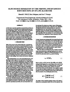
� P P 2 2 ! i jHii (! )j jsi (! )j SIR[H; s] = P P P : (14) 2 2 ! i j 6=i jHij (! )j hjsj (! )j i In the case of known channels and source signals we can compute the expressions directly by using a sample average over the available signal and multiplying the powers with the given direct and cross channel responses. We compared the performance of the proposed MAD algorithm to its corresponding o�-line counterpart [14], [15], and to a second decorrelation algorithm presented in [3]. This so-called transformed domain adaptive decorrelation algorithm (TDAD ) is a faster frequency domain implementation of the adaptive decorrelation algorithm presented by Weinstein et al. in [1]. It is based on decorrelating the covariance at a given time rather than at multiple times. As a result in principle it is not guaranteed to converge to the correct solution, but it has shown good performance in some simulated environments for a two source and two microphone case [3]. The most important question to address here is the adaption speed of the algorithm. The multi-path channel may Fig. 1. Test sequences for the simulated room (see main text). These are fteen-second speech and music sources sampled at 8 kHz. change very rapidly with moving sources. In particular Forty di�erent sections of varying length were used to estimate with fast head movements of a human subject the room the SIR improvements. response for that speaker may change quite abruptly. The question therefore is how much signal is required for MAD if the multi-path channel has completely changed. We used one simulated room response and one real room recording with a few seconds of signal each at 8 kHz. In all instances the separation lters where 2048 taps. In both the simulated and real room recordings 40 randomly-chosen segments out of 15-second signals where used ( gure 1 and 2). The mean and standard deviation for varying signal length are reported in gure 3 and gure 4. From these graphs we can conclude the following: 1. As expected we see that with increasing signal length the performance of MAD increases. 2. In all cases not more than a few seconds (3s-6s) of signal are required in order to converge to the best achievable performance. Within the margin of signal dependent variation in these particular environments the performance of MAD approaches that of the o�-line algorithm within approximately 3.5s. 3. The TDAD algorithm is very dependent on the signal. It's average performance is considerably better than our algorithm for the simulated room but it fails for our recording in a real room. This observation is consistent with the results reported in [3] on simulated environments and with the theoretical considerations on convergence to correct solutions [2]. The simulated room was computed using the algorithms of [25]2, with 2048 lter taps at 8 KHz (256 ms). We re- Fig. 2. Two separated speech signals recorded in a real o�ce environment. These particular results corresponds to a 15 dB SIR stricted the current experiments to the case of two sources improvement from 0.25 dB before separation. In the rst fteen and two microphones. The test signals consisted of a subseconds the speakers alternately spoke short digits. Because of ject counting digits and a music source (see gure 1), to the alternation, we could use this period to measure cross-talk source signals
0
5
10
15
seconds
separateded signals
0
We thank Joseph G. Desloge and Michael P. O'Connell of the Sensory Communication Group, Research Laboratory of Electronics, Massachusetts Institute of Technology for the software implementation in MATLAB. 2
5
10
15 seconds
20
25
30
power. Forty random sections of the last fteen seconds were used for training.
5
Start−Up performance for separation of two sources in simulated room 12
10
SIR improvement in dB
8
6
4
2
0
1
2
3
4 signal length in s
5
6
7
Fig. 3. Average SIR improvement before and after separation with the MAD (solid line) and TDAD (dashed line) algorithms in a simulated o�ce environment with two microphones and two sources (see text). The bars represent the standard deviation obtained by running the algorithms on 40 di�erent sections of the signal. The data-point on the very right represents the performance of the o�-line multiple decorrelation algorithm.
Start−Up performance for separation of two sources in real room 10
8
V. Conclusion
SIR improvement in dB
6
4
2
0
−2
−4
provide a more or less continuous stream of signal without long interruptions. The room is a 5 m x 5 m x 3 m rectangle with the absorption characteristic of a typical o�ce room (carpet oor, sheet-rock or gypsum-board walls, and acoustic tiles in the ceiling). The two microphones are placed at one of the walls at a distance of two meters from each other. That wall was chosen to be anechoic in order to generate a directional characteristic for the microphones. The sources have been placed at a distance of 1.5 meters in front of the microphones The real room recordings were obtained in a quiet o�ce environment of about the same size. The rst fteen seconds of signal contain alternating speech and where used to measure the cross talk powers before and after separation. The second fteen seconds of signal were used for training. In the end of the previous section we pointed out that it might be advantageous for the block algorithm to use larger frame rates, though the computational cost is higher. In particular for realistic environments we are using lters of considerable length (256 ms). Updating at a slower frame rate might not be su�cient. In TDAD a frame rate of r = 1 is used. In the previous experiments our MAD algorithm used a frame rate of r = 16, which results in an update of the cross-correlation and lter coe�cients every 16 ms. In order to choose the frame rates we determined the SIR improvements for the same real-room recordings as before for varying frame rates. In gure 5 we see that increasing the frame rate will in fact improve the performance. For this particular signal and environment a frame rate of 8 seems su�cient. Finally we want to note the implementation of this algorithm in C runs in real time on a 155 kHz Intel Pentium processor for a 2 input, 2 sources problem with a frame rate of 8 at 8 kHz sampling rate and T=2048
1
2
3
4 signal length in s
5
6
7
Fig. 4. Average SIR improvement before and after separation with the on-line MAD (solid line) and TDAD (dashed line) algorithms for real room recordings with two microphones and two sources (see text). The bars represent the standard deviations obtained by running the algorithms on forty di�erent sections of the signal. The data-point on the far right is the performance of the o�-line multiple decorrelation algorithm.
A key result of this work is that an on-line sourceseparation algorithm which supposedly exploits multiple decorrelation can visit the signals only once and yet within three-to-four seconds achieve the same separation performance as an o�-line multiple-decorrelation algorithm. At any time the on-line algorithm has only one estimate of the cross-correlation matrix. This stands in contrast to the o�line algorithm that diagonalizes multiple cross-correlation matrices by repeatedly accessing their values, which is equivalent to revisiting the data many times. Both algorithms assume non-stationarity of the signal so that multiple decorrelations provide su�cient conditions to unambiguously separate the sources. However in the on-line algorithm the multiple decorrelations are facilitated through a stochastic gradient that diagonalizes a changing average cross-correlation. To our knowledge this di�ers from all previous adaptive decorrelation algorithms, which drop the explicit averaging of the single cross-correlation matrix to get a stochastic update rule.
6
Dependence on frame rate at fixed signal length (3 sec) 10
[15] 9.5
[16] SIR improvement in dB
9
[17] 8.5
[18] 8
[19] 7.5
7
6.5
0
5
10
15
20
25
30
35
[20] [21]
frame rate
Fig. 5. Dependence of the MAD algorithm on the number of gradient [22] updates per signal block size ( lter size). For these results a [23] lter length of 2048 taps was used. At 8 kHz a frame rate of 4 corresponds to an update every 64 ms.
[1] [2] [3] [4] [5] [6] [7] [8] [9] [10] [11] [12] [13] [14]
[24] References E. Weinstein, M. Feder, and A.V. Oppenheim, \Multi-Channel [25] Signal Separation by Decorrelation", IEEE Trans. Speech Audio Processing, vol. 1, no. 4, pp. 405{413, Apr. 1993. S. Van Gerven and D. Van Compernolle, \Signal Separation by Symmetric Adaptive Decorrelation: Stability, Convergence, and Uniqueness", IEEE Trans. Signal Processing, vol. 43, no. 7, pp. 1602{1612, July 1995. K.-C. Yen and Y. Zhao, \Improvements on co-channel separation using ADF: Low complexity, fast convergence, and generalization", in Proc. ICASSP 98, Seattle, WA, 1998, pp. 1025{1028. M. Kawamoto, \A method of blind separation for convolved non-stationary signals", Neurocomputing, vol. 22, no. 1-3, pp. 157{171, 1998. S. Van Gerven and D. Van Compernolle, \Signal separation in a symmetric adaptive noise canceler by output decorrelation", in Proc. ICASSP 92, 1992, vol. IV, pp. 221{224. D. Yellin and E. Weinstein, \Multichannel Signal Separation: Methods and Analysis", IEEE Trans. Signal Processing, vol. 44, no. 1, pp. 106{118, 1996. H.-L. N. Thi and C. Jutten, \Blind source separation for convolutive mixtures", Signal Processing, vol. 45, no. 2, pp. 209{229, 1995. V. Capdevielle, C. Serviere, and J.L. Lacoume, \Blind separation of wide-band sources in the frequency domain", in Proc. ICASSP 95, 1995, pp. 2080{2083. S. Shamsunder and G. Giannakis, \Multichannel Blind Signal Separation and Reconstruction", IEEE Trans. Speech Audio Processing, vol. 5, no. 6, pp. 515{528, Nov. 1997. S. Cruses and L. Castedo, \A Gauss-Newton method for blind separation of convolutive mixtures", in Proc. ICASSP 98, Seattle, WA, 1998. R. Lambert and A. Bell, \Blind Separation of Multiple Speakers in a Multipath Environment", in Proc. ICASSP 97, 1997, pp. 423{426. S. Amari, S.C. Douglas, A. Cichocki, and A.A. Yang, \Multichannel blind deconvolution using the natural gradient", in Proc. 1st IEEE Workshop on Signal Processing App. Wireless Comm., 1997, pp. 101{104. T. Lee, A. Bell, and R. Lambert, \Blind separation of delayed and convolved sources", in Proc. Neural Information Processing Systems 96, 1997. L. Parra, C. Spence, and B. De Vries, \Convolutive Blind Source Separation based on Multiple Decorrelation", in IEEE Work-
shop on Neural Networks and Signal Processing, Cambridge, UK, September 1998, also presented at 'Machines that Learn' Workshop, Snowbird, April 1998. L. Parra and C. Spence, \Convolutive blind source separation of non-stationary sources", IEEE Trans. Signal Processing, 1999, accepted. N. Murata, S. Ikeda, and A. Ziehe, \An approach to blind source separation based on temporal structure of speech signals", IEEE Trans. Signal Processing, submitted. J. Principe, \Simultaneous diagonalization in the frequency domain (SDIF) for source separation", in ICA'99, Cardoso, Jutten, and Loubaton, Eds., 1999, pp. 245{250. K.-C Yen and Y. Zhao, \Adaptive Co-Channel Speech Separation and Recognition", IEEE Trans. Signal Processing, vol. 7, no. 2, March 1999. S. Amari, C.S. Douglas, A. Cichocki, and H.H. Yang, \Novel On-Line Adaptive Learning Algorithms for Blind Deconvolution Using the Natural Gradient Approach", in Proc. 11th IFAC Symposium on System Identi cation, Kitakyushu City, Japan, July 1997, vol. 3, pp. 1057{1062. P. Smaragdis, \Blind separation of convolved mixtures in the frequency domain", Neurocomputing, vol. 22, pp. 21{34, 1998. T. Ngo and N. Bhadkamkar, \"Adaptive blind separation of audio sources by a physically compact device using second-order statistics"", in ICA'99, Loubaton Cardoso, Jutten, Ed., 1999, pp. 257{260. H. Sahlin and H. Broman, \Separation of real-world signals", Signal Processing, vol. 64, pp. 103{104, 1998. P. Nelson, F. Orduna-Bustamante, and H. Hamada, \Inverse lter design and equalization zone in multichannel sound reproduction", IEEE Trans. Speech Audio Processing, vol. 3, no. 3, pp. 185{192, May 1995. D Brandwood, \A complex gradient operator and its application in adaptive array theory", IEE Proc., vol. 130, no. 1, pp. 11{16, Feb. 1983. P.M. Peterson, \Simulating the response of multiple microphones to a single acoustic source in a reverberant room", J. Acoust. Soc. Am., vol. 80, no. 5, pp. 1527{1529, Nov. 1986.