Range-Free Localization Schemes for Wireless Sensor Networks

World Academy of Science, Engineering and Technology International Journal of Computer, Electrical, Automation, Control and Information Engineering Vol:9, No:7, 2015

Range-Free Localization Schemes for Wireless Sensor Networks R. Khadim, M. Erritali, A. Maaden 

International Science Index Vol:9, No:7, 2015 waset.org/Publication/10002217

Abstract—Localization of nodes is one of the key issues of Wireless Sensor Network (WSN) that gained a wide attention in recent years. The existing localization techniques can be generally categorized into two types: range-based and range-free. Compared with rang-based schemes, the range-free schemes are more costeffective, because no additional ranging devices are needed. As a result, we focus our research on the range-free schemes. In this paper we study three types of range-free location algorithms to compare the localization error and energy consumption of each one. Centroid algorithm requires a normal node has at least three neighbor anchors, while DV-hop algorithm doesn’t have this requirement. The third studied algorithm is the amorphous algorithm similar to DV-Hop algorithm, and the idea is to calculate the hop distance between two nodes instead of the linear distance between them .The simulation results show that the localization accuracy of the amorphous algorithm is higher than that of other algorithms and the energy consumption does not increase too much.

Keywords—Wireless Sensor Networks, Node Localization, Centroid Algorithm, DV–Hop Algorithm, Amorphous Algorithm.

W

I. INTRODUCTION

IRELESS SENSOR NETWORK (WSN) is composed of a large number of sensor nodes, which have the ability of sensing, computation, and wireless communication and can monitor and acquire physical information in the distribution detection area in real time. WSN have attracted worldwide research and industrial interest, because they can be applied in various areas such as hospital surveillance, smart home, and environmental monitoring. For most of these applications, localization is a fundamental issue, because users normally need to know not only what happens, but also where interested events happen or where the target is [1]. For example, in hospital surveillance, the knowledge of where the patient can help the doctors to arrive at the right place as quickly as possible in urgent case [2], [3]; in a disaster relief operation using WSN to locate survivors in a collapsed building, it is critical that sensors report monitoring information along with their location [4][7]. On the other hand, the position parameters of sensor nodes are assumed to be available in many operations for network management, such as routing where a number of geographical algorithms have been proposed [8]-[10], topology control that R. Khadim and A. Maaden are with Laboratory of Mathematics and Applications, Faculty of Sciences and Techniques, Sultan Moulay Slimane University. M. Erritali is with TIAD laboratory, Computer Sciences Department, Faculty of sciences and techniques, Sultan Moulay Slimane University, BeniMellal, BP: 523, Morocco (phone: +212670398838; e-mail: [email protected]).

International Scholarly and Scientific Research & Innovation 9(7) 2015

uses location information to adjust network connectivity for energy saving [11]-[13]. The location of sensor nodes is not predetermined or engineered. This allows that sensor nodes can be deployed randomly in inaccessible terrains or disaster relief operations. On the other hand, this also means that sensor network protocols and algorithms must possess self-organizing capabilities [14]. In WSNs the localization problem can be intercepted that in a sensor network, the location of multiple nodes has been known (beacon node) and the location of target node (unknown nodes) is obtained by the sensor information and effective localization algorithm [15]. At present, many ideas have been proposed for node localization in wireless sensor networks [16]-[19]. According to whether or not the network needs to measure the actual distances between network nodes and based on whether accurate ranging is required, WSN localization algorithm can be divided into two categories: Range-Based algorithm and Range-Free algorithm. The Range-based schemes [20]-[24] algorithm mainly includes the measurements of angle and distance (the range information) such as Received Signal Strength Indicator (RSSI) [24], Time of Arrival (TOA) [22], Time Difference on Arrival (TDOA), and Angle of Arrival (AOA) [24], [25], between concerned equipment, and then the calculate the desired position based on trilateration or triangulation approaches. So it needs extra hardware supporting, large computing and communicating with high energy consumption. While the range-based scheme uses the distance or angle between nodes, the range-free approach only depends on the connectivity information between nodes such as the hops for localization without any extra hardware supporting [26]. In this scheme, the nodes that are aware of their positions are called anchors, while others are called normal nodes. Anchors are fixed, while normal nodes are usually mobile. Normal nodes first gather the connectivity information as well as the positions of anchors, and then calculate their own position [27]. The connectivity information of a node N can be its hop counts to other nodes. The connectivity is used as an indication of how close this node N to other nodes .Since no ranging information is needed the range-free scheme can be implemented on low-cost wireless sensor networks. Another advantage of the range-free scheme is its robustness; the connectivity information between nodes is not easily affected by the environment [28]. Although the localization accuracy of the range-based algorithm is usually higher than that of the range-free Algorithm because of the simple hardware support,

1452


the lower consumption, and the antinoise ability, the rangefree algorithm is widely used in many applications. As a result, we focus our research on the range-free scheme. The range-free algorithm includes Centroid algorithm, Distance Vector-Hop (DV-Hop), and Amorphous algorithm. It includes Centroid algorithm [29], Distance Vector-Hop (DV-Hop) [30], and Amorphous algorithm [31].


II. LOCALIZATION ALGORITHMS A. Centroid algorithm Bulusu and Heidemann [29] have proposed the centroid localization algorithm, which is a range-free, proximity-based, coarse-grained localization algorithm. The algorithm implementation contains three core steps. First, all anchors send their positions to all sensor nodes within their transmission range. Each unknown node listens for a fixed time period t and collects all the beacon signals it receives from various reference points. Second, all unknown sensor nodes calculate their own positions by a centroid determination from all n positions of the anchors in range. The centroid localization algorithm uses anchor nodes (reference nodes), containing location information x , y to estimate node position. After receiving these beacons, a node estimates its location using the following centroid formula: xest ,yest

x1 x2 … xk k

,

y1 y2 … yk k

(1)

B. DV-Hop algorithm DV-hop is a distributed hop by hop positioning algorithm proposed by Dragos Niculescu and Badri Nath [30]. This is the most basic scheme; it uses an exchange distance vector so that all nodes in the network are able to calculate the distance between the anchors. Each anchor maintains a table , , where , are the coordinates of other network anchors and is the number of hops separating the latter from the node. Each anchor calculates the distance to the other anchors in the network, using the location information obtained from a positioning system; it deduces an approximation of the hop distance. This is the hop distance that will constitute the correction information for the entire network. Each anchor node calculates: Hopsizei

∑i#j

xi ‐xj

2

yi ‐yj

x x x

to unknown nodes, and then we y y y y ⋮ y y

x x x

d d d

(4)

Formula (5) can be schemed with the following linear equation: AP

(5)

B

Where (6)

P

A

x x

2∗

x x

y y

⋯

d d

d d

(7)

⋯ x

x

B=

y y

x x

y

y

x x

y y

y y

(8)

⋮ d

d

x

x

y

y

The position of the unknown node is obtained by using least square method, which can be expressed as: A A

P

(9)

A B

C. Amorphous Algorithm Amorphous algorithm is similar to DV-Hop algorithm, and the idea is to calculate the hop distance between two nodes instead of the linear distance between them. Amorphous algorithm is composed of the following three steps [32]. 1. Calculate the Minimum Hop from the Unknown Node to the Beacon Node. Every beacon node sends messages to the unknown nodes by flooding method. Formula (10) is used to calculate the minimum hop from the node to .

∑ ,

,

|

,

|

0.5

(10)

2

∑i#j hij

(2)

After all unknown nodes have received the hop-size from anchor nodes which have the least hops between them; they compute the distance to the anchor nodes based on two factors: hop-size and minimum hop count h using: d

distance between anchors have:

h ∗ HopSize

(3)

In the third step, unknown nodes calculate their position according to the distance to each anchor node obtained in the second step. Let x, y be the coordinates of the unknown node, and x , y the coordinates of anchor . Let’s say d is the


Where:

is the minimum hop from the unknown node is the integer hop from the , unknown node to the beacon node ; , is the integer hop : are from the unknown node to the beacon node ; |:is the the neighbor nodes around the unknown node ; | number of the neighbor nodes around the unknown node . ,

to the beacon node ;

2. Calculate the Distance from the Unknown Node to the Beacon Node Formula (11) is used to calculate the average distance of one hop:

1453


2 1 ‐ nlocal ⁄π arcos t‐t 1‐t e ‐1

HopeSize r 1 e‐nlocal ‐

III. EXPERIMENTAL RESULTS dt

(11)

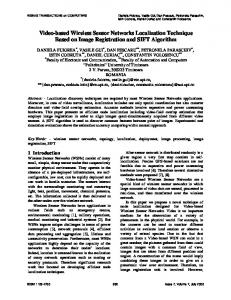
A. Network Topology The network topology is an isotropic topology:

where is the wireless range of the node and is the average connectivity of the network. The distance from the unknown node to the beacon node can be calculated on the basis of the average distance of one hop and the minimum hop from the unknown node to the beacon node [31]. It can be expressed: (12)


,

3. Adopt the Least Squares Method to Locate When the estimated distances from the unknown node to three or more than three beacon nodes have been obtained, the location of the unknown node can be calculated. It is shown as: y ⋮ y

x x

d d

(13)

The above formula will be solved by the least squares method; the location of the unknown node can be obtained:

A A

X

(14)

A b

, , …… where , , , , are the coordinates of beacon nodes, , is the coordinates of the unknown , , ,…., are the distances from node, and the unknown node to the beacon nodes: x A x

2∗ x

x

y

⋯

y ⋯

x

x y

y

y

y d

d

⋮

B= x

x

y

y

(15)

(16)

Fig. 1 Network isotropic topology

B. The Simulation Platform and Distribution of Nodes MATLAB simulation software can be used to verify the feasibility of the algorithms. Network deployment area is 1000 m × 1000 m, the node coordinates are generated randomly, the number is 300, there are 60 beacon nodes, the proportion of beacons is 20%, the wireless range is 300 m, and communication model is Regular Model. Distribution of nodes is shown in Fig. 2. C. Localization error The localization error is an important indicator to evaluate the localization performance. To calculate the localization error we use:

d d

The location of the unknown node can be calculated on the basis of (15) and (16).


(17)

where x , y is the actual location of the unknown node and x ,y is the estimated location, where R is the wireless range.

1454



Fig. 2 Distribution of nodes figures: (a) Centroid algorithm (b) DV-Hop algorithm (c) Amorphous algorithm

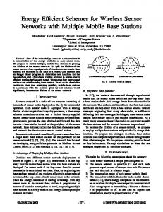
D.Simulation of Different Algorithms The different algorithms can be simulated to get the localization error shown in Fig. 3. In Fig. 3, the little blue circle represents the estimated location of the unknown node and the blue line represents the localization error of the unknown node.


The localization error of Centroid algorithm is 0, 2937. The localization error of DV-Hop algorithm is 0, 3022. The localization accuracy of the Centroid algorithm is higher than that of the DV-Hop algorithm. The localization error of Amorphous algorithm is 0, 2361. We can see that the localization accuracy of the amorphous algorithm is higher than that of the centroid algorithm and DV-Hop algorithm obviously.

1455



Fig. 3 The localization error figures: (a) Centroid algorithm, (b) DV-Hop algorithm, and (c) Amorphous algorithm

E. The Simulations under Different Conditions Are Completed for the Three Algorithms To find the performance of the different algorithms proposed in this paper. The simulations under different conditions are completed for Centroid, DV-Hop, and Amorphous. All the nodes in the simulation are randomly distributed in the area 1000 m × 1000 m. Each set of the condition is run for 1000 times so as to actually reflect the localization error of different algorithms. The average value of the localization error is used for the comparison. In the condition of different proportions of beacons, there are 300 nodes in total with the wireless range being set as 300m. From Fig. 4 (a), it is clear that the localization error of the three algorithms decreases as the proportion of beacons increases. In the simulation of different wireless range, the proportion of beacons is set by 20% and the total number of nodes is set by 300. Fig. 4 (b) shows the result of the simulation. It is clear that the localization error of the algorithms decreases as the wireless range increases. The localization error of the amorphous algorithm increases when wireless range is more than 300m. Based on different numbers of nodes, wireless range is set as 300m, and the proportion of beacons is set as 20%. The


result is shown in Fig. 4 (c). It is clear that the localization error of the 3 algorithms decreases as the number of nodes increases. F. The Computing Time of Different Algorithms Computational costs make up only a small part of all energy consumption in WSN; most of the energy consumption is communication. So decreasing the energy consumption of communication is the key to extend the lifecycle of network. In order to decrease the energy consumption of communication, all nodes cannot send the information to a central node to calculate their location, because the energy consumption of communication is too large. Table I compares the average computing time needed by the three algorithms to localize a single node and localization error. All experiments are conducted on the same computer. Network deployment area is 1000 m × 1000 m, the node coordinates are generated randomly, the number is 300, the proportion of beacons is 20%, the wireless range is 300 m, and communication model is Regular Model. Due to the simple calculation, Centroid algorithm generally requires less computing time than the other four algorithms. Amorphous algorithm is similar to DVHop algorithm.

1456



Fig. 4 The localization error under different conditions: (a) proportion of beacons and localization error, (b) wireless range and localization, (c) number of nodes and localization error TABLE I AVERAGE COMPUTING TIME TO LOCALIZE SINGLE NODE AND LOCALIZATION ERROR algorithms localization error computing time centroid 0.2937 0.383 dv-hop 0.3022 0.512 amorphous 0.2361 0.536

G.The Energy Consumption To find out the performance of the algorithm proposed in this paper, the simulations of energy consumption under different conditions are completed for Centroid, DV-HOP and Amorphous algorithm. All the nodes in the simulation are randomly distributed in the area 1000 m × 1000 m. Each set of the condition is run for 1000 times so as to factually reflect the energy consumption of different algorithms. In the condition of different proportions of beacons, there are 300 nodes in total with wireless range being set as 300 m. The result of energy consumption is shown in Fig. 5 (a). It is clear that


energy consumption of the three algorithms increases as the proportion of the beacons increases. Under the same proportion of beacons, the energy consumption of Centroid algorithm is lowest, because it broadcasts only once. DV-hop algorithm needs to broadcast twice, so the energy consumption of communication is large [13]. In the case of different wireless range, there are 300 nodes in total with proportion of beacons being set as 20%, and in the case of different numbers of nodes, wireless range is set as 300 m, the proportion of beacons is set as 20%. The similar result can be got in Figs. 5 (b) and (c). It is certain that accurate localization will bring more energy consumption. So localization algorithm should be designed according to different applications.

1457



Fig. 5 Energy consumption under different conditions: (a) energy consumption on different proportions of beacons, (b) consumption on different wireless range, and (c) energy consumption on different numbers of nodes

REFERENCES

IV. CONCLUSION Positional accuracy is very important indicator for assessing the location of performance. More localization is high precision location of the performance is better. A conclusion might elaborate on the importance of the work or suggest applications and extensions. In addition, the accuracy of the location of the amorphous algorithm is superior to that of other algorithms and there is not a large increase of energy consumption, which is why it is suitable for the location of network nodes large scale.

[1] [2] [3]

[4] [5]

ACKNOWLEDGMENT This research was supported by The Laboratory of Mathematics and Applications, Faculty of Sciences and Techniques, Sultan Moulay Slimane University Beni Mellal Morocco. We thank our colleagues from Tiad laboratory, Department of Computer Sciences, Faculty of Sciences and Techniques, Sultan Moulay Slimane University who provided insight and expertise that greatly assisted the research.


[6] [7]

[8]

1458

Linqing Gui, Improvement of Range-free Localization Systems in Wireless Sensor Networks, PhD thesis, 13 February 2013 Y. Lee, W. Chung “Wireless sensor network based wearable smart shirt for ubiquitous health and activity monitoring”, Sensors and Actuators B: Chemical, vol: 140, issue: 2, pp: 390-395, 16 July 2009. G. López, V. Custodio, J. Moreno, "LOBIN: E-Textile and WirelessSensor-Network Based Platform for Healthcare Monitoring in Future Hospital Environments," IEEE Transactions on Information Technology in Biomedicine, vol.14, no.6, pp.1446-1458, Nov. 2010. G. Werner-Allen, K. Lorincz, et al. “Deploying a wireless sensor network on an active volcano”. IEEE Internet Computing, vol. 10, no. 2, pp. 18-25, Mar. 2006. J. Li, M. Yu, “Sensor coverage in wireless ad hoc sensor networks”, International Journal of Sensor Networks, vol. 2, no. 3/4, pp. 218-229, Jun. 2007. M. L. Lazos, R. Poovendran, “SeRLoc: Robust localization for wireless sensor networks”, ACM Transactions on Sensor Networks, vol. 1, no. 1, pp. 73-100, Aug. 2005. A. Terzis, A. Anandarajah, K. Moore, et al. “Slip surface localization in wireless sensor networks for landslide prediction”, In Proceedings of the 5th international Conference on information Processing in Sensor Networks (IPSN ‘06), Nashville, Tennessee, USA, April 19-21, 2006, pp. 109-116. S. Basagni, I. Chlamtac, V. Syrotiuk, et al. “A distance routing effect algorithm for mobility (DREAM)”, In Proceedings of the 4th Annual ACM/IEEE international Conference on Mobile Computing and Networking (MobiCom ‘98), Dallas, Texas, USA, Oct. 25-30, 1998, pp. 76-84.


[9]

[10]

[11] [12] [13]

[14]


[15] [16]

[17] [18]

[19] [20]

[21]

[22]

[23]

[24] [25]

[26]

[27]

[28] [29]

B. Karp, H. Kung, “GPSR: greedy perimeter stateless routing for wireless networks”, In Proceedings of the 6th Annual international Conference on Mobile Computing and Networking (MobiCom ‘00), Boston, Massachusetts, USA, Aug. 06-11, 2000, pp. 243-254. Y. Kim, R. Govindan, B. Karp, et al. “Geographic routing made practical”, In Proceedings of the 2nd Conference on Symposium on Networked Systems Design and Implementation (NSDI ‘05), May 0204, 2005, Berkeley, CA, USA, pp. 217-230. K. Alzoubi, X. Li, Y. Wang, et al. “Geomet IEEE Transactions on Parallel and Distributed Systems, vol. 14, no. 4, Apr. 2003, pp. 408-421. N. Li, J. Hou, “Localized topology control algorithms for heterogeneous wireless Networks”, IEEE/ACM Transactions on Networking, vol. 13, no 6. 2005, pp. 1313-1324. Y. Xu, J. Heidemann, D. Estrin, “Geography-informed energy conservation for Ad Hoc routing”. In Proceedings of the 7th Annual international Conference on Mobile Computing and Networking (MobiCom ‘01), Rome, Italy, Jul. 16-21, 2001, pp. 70-84. F. Akyildiz, W. Su, Y. Sankarasubramaniam, and E. Cayirci, “Wireless sensor networks: a survey,” Computer Networks, vol. 38, no. 4, pp. 393– 422, 2002. L. Haibo, W. Yingna, and P. Bao, “A Localization method of Wireless sensor network based on two-hop focus,” Procedia Engineering, vol. 15, pp. 2021–2025, 2011. V. Chandrasekhar, et al. “Localization in underwater sensor networks: survey and challenges”. In Proceedings of the 1st ACM international Worksh(WUWNet ‘06), Los Angeles, CA, USA, Sep. 25, 2006, pp. 3340. G. Mao, B. Fidan, B. Anderson, “Wireless sensor network localization techniques”. Computer Networks, vol. 51, no. 10, Jul. 2007, pp. 25292553. I. Amundson, and X. Koutsoukos, “A survey on localization for mob networks”. In Proceedings of the 2nd international Conference on Mobile Entity Localization and Tracking in GPS-Less Environments, Orlando, FL, USA, Sep. 30, 2009, pp. 235-254. Y. Liu, Z. Yang, X. Wang, et al. “Location, Localization, Localizability”. Journal of Computer Science and Technology, vol. 25, no. 2, Mar. 2010, pp. 247-297. R. Ouyang, A. Wong, K. Woo, "GPS Localization Accuracy Improvement by Fusing Terrestrial TOA Measurements", IEEE International Conference on Communications (ICC), pp. 1-5, May 2010. P. Kumar, L. Reddy, S. Varma, “Distance measurement and error estimation scheme for RSSI based localization in Wireless Sensor Networks,” Fifth IEEE Conference on Wireless Communication and Sensor Networks (WCSN), Allahabad, India, pp. 1-4, Dec. 2009 P. Voltz, D. Hernandez, “Maximum likelihood time of arrival estimation for real-time physical location obile stations in indoor environments,” Position Location and Navigation Symposium (PLANS), California, USA, pp. 585-591, April 2004. L. Kovavisaruch, and K. Ho, “Alternate source and receiver location estimation using TDOA with receiver position uncertainties,” IEEE International Conference on Acoustics, Speech, and Signal Processing (ICASSP '05), Pennsylvania, USA, pp. iv/1065 - iv/1068, March 2005. P. Rong, and M. Sichitiu, “Angle of arrival localization for wireless sensor networks,” Annual IEEE Communications Society on Sensor and Ad Hoc Communications and Networks, USA, 2006, vol.1, pp.374-382. J. Yao, J. Li, L. Wang, and Y. Han, “Wireless sensor network localization based on improved particle swarm optimization,” in Proceedings of the International Conference on Computing, Measurement, Control and Sensor Network (CMCSN ’12), pp. 72–75, July 2012. Linqing GUI, Thierry VAL, Anne WEI, “An Adaptive Range-free Localization Protocol in Wireless Sensor Networks”, International Journal of Ad Hoc and Ubiquitous Computing, in review, submitted on 20 December 2012. Linqing Gui, Thierry Val, Anne Wei, Réjane Dalce, “Improvement of Range-free Localization Systems Realized by a DV-hop Protocol in Wireless Sensor Networks”, Ad Hoc & Sensor Wireless Networks, in review, submitted on 5 July 2012. Linqing Gui, Anne Wei, Thierry Val, “A Range-Free Localization Protocol for Wireless Sensor Networks”, International Symposium on Wireless Communications Systems, Paris, August 2012 N. Bulusu, J. Heidemann and D. Estrin, GPS-less Low Cost Outdoor Localization for Very Small Devices, IEEE Personal Communications Magazine, 7(5):28-34, October 2000.


[30] D. Niculescu and B. Nath, DV Based Positioning in Ad hoc Networks, In Journal of Telecommunication Systems, 2003. [31] R. Nagpal, H. Shrobe, J. Bachrach, Organizing a Global Coordinate System from Local Information on an Ad Hoc Sensor Network, In the 2nd International Workshop on Information Processing in Sensor Networks (IPSN '03), Palo Alto, April, 2003. [32] Y. Liu, “An adaptive multi-hop distance localization algorithm in WSN,” Manufacturing Automation, vol. 33, pp. 161–163, 2011 R. Khadim was born in Beni Mellal, Morroco in September 1991, received the fundamental license in physics (option electronics and industrial systems), and master of Business Intelligence degrees from Soltan Moulay Sliman’s University, Beni-Mellal, Morroco in 2012 and 2014 respectively. Her general interests span the areas of Localization and mobility of ad-hoc sensor networks. She can be contacted at: [email protected]. M. Erritali obtained a master's degree in business intelligence from the faculty of science and technology, Beni Mellal at Morocco in 2010 and a Ph.D. degree in Computer Sciences from the faculty of sciences, Mohamed V Agdal University, Rabat, Morocco in 2013. His current interests include developing specification and design techniques for use within Intelligent Network, data mining, information Retrieval, image processing and cryptography. He is currently a professor at the Faculty of Science and Techniques, University Sultan Moulay Slimane, and also a member of the TIAD laboratory. He can be contacted at: [email protected]

1459

Range-Free Localization Schemes for Wireless Sensor Networks

Range-Free Localization Schemes for Wireless Sensor Networks

Suggest Documents

A Taxonomy of Localization Schemes for Wireless Sensor Networks

Localization Systems for Wireless Sensor Networks

Indoor Localization for Wireless Sensor Networks - Embedded ...

Localization of Distributed Wireless Sensor Networks ...

LOCALIZATION IN WIRELESS SENSOR NETWORKS Mark Terwilliger ...

Wireless Sensor Networks Localization Methods - arXiv

Video-based Wireless Sensor Networks Localization ... - wseas.us

wireless sensor networks localization algorithms: a

Shooter Localization in Wireless Sensor Networks

INDOOR LOCALIZATION WITH WIRELESS SENSOR NETWORKS SA ...

Localization in Wireless Sensor Networks - CiteSeerX

Localization in Wireless Sensor Networks - Semantic Scholar

Wireless Sensor Networks Chapter 9: Localization ...

Multistage Localization in Wireless Sensor Networks ...

Energy efficient schemes for wireless sensor networks ... - Google Sites

Energy efficient schemes for wireless sensor networks with multiple ...

Energy efficient schemes for wireless sensor networks with multiple ...

Alternative Data Gathering Schemes for Wireless Sensor Networks

Localization Using Neural Networks in Wireless Sensor Networks

A New Methodology for Self Localization in Wireless Sensor Networks

Robust Node Localization for Wireless Sensor Networks - cs.Virginia

Probabilistic Localization for Wireless Sensor Networks - NC State

GPS-Free Localization Algorithm for Wireless Sensor Networks - MDPI

A Survey on Localization for Mobile Wireless Sensor Networks