Index TermsâLocalization, wireless sensor network, dis- ... of applications such as environmental monitoring, gathering .... The idea is simple, yet powerful.
Simple Algorithm for Outdoor Localization of Wireless Sensor Networks with Inaccurate Range Measurements Mihail L. Sichitiu, Vaidyanathan Ramadurai and Pushkin Peddabachagari Department of Electrical and Computer Engineering North Carolina State University Raleigh, NC 27695 email: {mlsichit,vramadu,ppeddab}@ncsu.edu
Abstract— We consider the problem of determining the positions of wireless nodes using range measurements from multiple, sparsely located, beacon stations with known locations. A large number of such nodes surrounding the beacon stations automatically and cooperatively estimate their position through collaborative efforts and iterative refinements. These positions are propagated to other nodes in the network, allowing the entire network to create an accurate map of itself. The proposed approach features robustness with respect to range measurement inaccuracies, low complexity and distributed implementation, using only local information. Index Terms— Localization, wireless sensor network, distributed, range inaccuracy, position estimates.
I. I NTRODUCTION Wireless ad-hoc sensor networks are being extensively used to study various aspects of the physical environment which are complex in nature. They are deployed for a wide range of applications such as environmental monitoring, gathering military intelligence, providing disaster reliefs, factory instrumentation and information tracking, etc. Data from these sensors is of very little use without corresponding position information. For example, in a forest fire it is very important to know where the actual event is detected. To determine the position of the nodes, they can be handplaced and their position carefully recorded (a tedious and error-prone method, completely impractical for a large number of sensor nodes); they can be equipped with GPS in an outdoor environment (a costly proposition in terms of volume, power and money); or alternatively, a localization algorithm can be used to localize them after deployment. In this paper, we explore the problem of localization in wireless sensor networks and propose a distributed algorithm that enables the nodes to establish confident position estimates in the presence of ranging inaccuracies. Any ad-hoc wireless network can use this solution to estimate the position of its nodes. The wireless sensor networks example is chosen because it illustrates a practical application of a potentially large network of very cheap nodes. This work was supported by a Faculty Research and Development Grant at NC State University.
The main limitation of the method is that it only works reliably in outdoor environments. The method is based on radio-frequency (RF) signal strength measurements, and outdoors, the signal propagation (as it was pointed before [1] and from our own measurements presented in Section II) is approximately circular (even in wooded environments). Indoors, walls would severely reduce the precision of the method due to nonlinearities, noise, interference and absorption [2]– [5]. However, many sensor networks will likely be deployed outdoors, and will be able to take advantage of the proposed approach. Many localization systems have been proposed and implemented [1]–[16]. Our approach, to the best of the authors’ knowledge, is the only one to consider inaccurate range measurements (encountered, especially, when using RSSI measurements) and to scale independently of the total number of nodes (i.e., O(1) in the total number of nodes in the network). The algorithm is RF based, leveraging the wireless transceiver already present in the nodes.
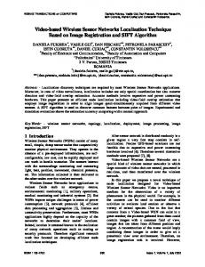
12
24 23
19
11 13 3
22 14
2
18
6
21
15 10
5
20 7
4
17 9
1
8
16
Fig. 1. Wireless ad-hoc network of 24 nodes. Nodes 3, 7, 13, 17 and 23 are beacons (with known positions). Different transmission ranges correspond to different concentric rings around the beacon nodes.
II. P ROBLEM F ORMULATION Fig. 1 depicts a wireless ad-hoc network of 24 nodes. A line between two nodes shows that the nodes are within the transmission range of each other. Each node belongs in one of two classes: beacons and unknown nodes. The beacons are the black nodes 3, 7, 13, 17 and 23. We assume that these beacons have known positions (either by being placed at known positions, or by using GPS). We will refer to the GPS-less nodes as unknown nodes [10]. We assume that a range measurement method is available (we elaborate later in this paper on a few options). Thus, an unknown node receiving a packet from a beacon (or from another unknown node) will be able to determine (with some confidence) that it is positioned somewhere within the ring defined by the circles of radii Ri−1 and Ri and centered at the beacon (or at the other unknown node). In Fig. 1, corresponding to different ranges we have different concentric rings around the beacon nodes. We will refer to the packets meant to assist unknown nodes in establishing their position estimates as beacon packets. Distance, or range measurement can be achieved in several different ways. One ranging method relies on measuring the propagation delay of an ultrasonic impulse sent by the beacons simultaneously with a radio packet [9], [10]. A different method of measuring the range is through received signal strength indicator (RSSI) measurement (virtually all currently available transceivers support it). While this method is not as accurate as the acoustic one, it doesn’t require any extra equipment. As in the acoustic case, unless the nodes are outdoors with no obstacles, the range measurement is not reliable; however, if the nodes are outdoors with no obstructions, the model of a uniform, circular range holds surprisingly well [1]. To evaluate the accuracy of RSSI measurements, we used two Lucent Orinoco IEEE 802.11b cards on two laptops to measure the signal strength as a function of the distance between them. One of the laptops was configured to continuously send beacon packets, and the other one measured the signal strength for each received packet (we used the packet capture library - pcap - and the monitor mode of the Lucent Orinoco card). Two sets of measurements were taken, one in a relatively open space (Fig. 2(a)) and another in a thickly wooded area (Fig. 2 (b)). Measurements performed in this manner can be used effectively for ranging. For example, in Fig. 2(b), if the mean of several received packets is 84, then we can conclude with high confidence that the sender is somewhere between 7 m and 14 m. One can combine the signal strength measurement with transmission at different power levels for an increased accuracy in range determination. In this case, a table with power level on the rows and RSSI on the columns can be used to find the minimum and maximum range to the transmitter of a beacon packet A graph similar to the one in Fig. 2 will be produced for each power level. The graph can be used to
TABLE I A N EXAMPLE OF RANGE INTERVAL DETERMINATION GIVEN THE POWER LEVEL AND THE RSSI OF A RECEIVED BEACON PACKET. Power Level 1 2 3 4
1 4m - 20m 8m - 30m 15m - 40m 40m - 70m
RSSI 2 3 1m - 10m 0 - 8m 5m - 15m 1m - 12m 10m - 30m 5m - 15m 25m - 50m 20 - 30m
4 0 - 5m 0 - 8m 0 - 10m 0 - 20m
generate the above-mentioned table. An example of such a table with two power levels and four RSSI values is presented in Table I. In a real implementation, the table will have an entry for every valid value of the RSSI (alternatively an interpolation scheme may be used). Range determination using power level and/or received signal strength indications is also susceptible to inaccuracies due to interference and multi-path fading due to obstacles; but, this uncertainty can be captured in the interval presented in Table I. The position estimation algorithm that will be introduced in the following sections is specifically geared to inaccurate range measurements. III. A D ISTRIBUTED P OSITION E STIMATION A LGORITHM In this section, a position estimation algorithm will be presented. The idea is simple, yet powerful. At first, we will consider the case of stationary nodes and a uniform range determination like the one presented in Table I. We consider that for each beacon packet received, an unknown node can infer that it is positioned somewhere on a ring around the node that sent the beacon packet.
MyID Power Level My Position Estimate Fig. 3.
The format of a beacon packet
The format of a beacon packet is shown in Fig. 3. Each such packet contains the id of the node from where the packet originates, the power level used to transmit this packet and the position estimate of the node transmitting this packet. In the case of beacons, the position estimate is a point (in the ideal case) or a very small area (corresponding to the uncertainty in GPS measurements).
14
7
13
10
Fig. 4. Unknown nodes 10 and 14 helping each other to improve their position estimates.
As a matter of fact, an unknown node can assist other unknown nodes in finding their position estimates as soon
110
110
100
Received Signal Strength Indicator
Received Signal Strength Indicator
100
90
80
70
80
70
60
60
50
90
0
5
10
15
20 Distance (m)
25
30
35
40
(a)
50
0
5
10
15
20 Distance (m)
25
30
35
40
(b)
Fig. 2. Outdoor received signal strength measurements as a function of the distance. (a) Measurements taken in an environment with no obstructions, (b) Measurements taken in a heavily wooded area.
as it has any kind of information about its own position by transmitting its position estimate enclosed in a beacon packet similar to the one transmitted by the real beacons. Consider the situation depicted in Fig. 4. If the two unknown nodes 10 and 14 do not help each other, they can only determine that they are somewhere on two rings centered at beacon nodes 7 and 13, respectively. If they communicate their position estimates to each other, they can improve each other’s estimates: they can determine that their positions are within the two dotted areas. Each unknown node in the network will execute the pseudocode shown in Fig. 5. 1. Initialize the position estimate to the entire space. 2. Receive beacon packet from a neighbor node (beacon or unknown node). 3. Update the position estimate. a. Compute the constraint from the beacon packet. b. Intersect the constraint with the current position estimate to get the new position estimate. 4. If at step 3 the position estimate improved (has a smaller area), then broadcast the updated position estimate to all neighbors. 5. Goto step 2. Fig. 5.
Pseudo-code of the position estimation algorithm
If the beacon packet at step 2 is coming from a beacon, it will contain the exact coordinates of the beacon with no uncertainty. If the message comes from an unknown node, it will contain the position estimate for that unknown node. At step 3, the position estimate is updated by computing the intersection between the current position estimate and the
constraints imposed by the beacon packet received at step 2. Formally expressed, the position estimate is updated as follows: N ewP ositionEstimate = OldP ositionEstimate ∩ N ewConstraint
(1)
Since intersection is used, the new position estimate may either be unchanged or it may improve; but, it will never be larger than the old one. When the received beacon packet comes from a beacon, the constraint is easy to define. It is just a ring centered at the beacon coordinates. The beacon coordinates are included in the beacon packet as “My Position Estimate”. When the packet comes from an unknown node, which has only an estimate of its position, the constraint is slightly more difficult to compute. To compute the new constraint, we need to compute the Minkowski sum [17] of the position estimate and the transmission ring. Given two surfaces S1 and S2 , their Minkowski sum is obtained by the union of all translations of S2 in each and every point of S1 . This is similar to the regular 1-D function convolution, and it has the same properties. S 2 ◦ S1 = S1 ◦ S2 =
[
S2 shifted to p
(2)
p∈S1
For example, the Minkowski sum of the surface shown in Fig. 6(a) with the surface shown in Fig. 6(b) is shown in Fig. 6(c). When computing the new constraint by Minkowski sum, we need the position estimate of the source (Fig. 6(a)) and the transmission range surface (Fig. 6(b)). The position estimate is explicitly included in the beacon packet. The transmission range is obtained from Table I; the power level is included in the beacon packet and RSSI is measured during the reception of the packet. Since the broadcast at step 4 is only performed if the position estimate improved, the algorithm will terminate in a
(a)
(b) Fig. 6.
(c)
(a) Surface 1, (b) Surface 2, (c) Minkowski sum of surface 1 and surface 2.
finite number of steps. A bound on the total number of steps will be provided in the next section. The algorithm described in this section has the following properties: • It is distributed and receiver based. • It is scalable as the algorithm has a linear complexity O(m) in the number of neighbors for each node and constant complexity O(1) with the total number of nodes. • It uses only local information. The information from distant beacon nodes degrades and gets discarded as it propagates; therefore, only information from nearby beacons will be used whenever possible. • It is robust to range measurement inaccuracies and transmission errors. • It has reduced complexity. In the proposed solution, each node will store a very small state (its position estimate), which ensures that the implementation is possible on a large variety of hardware platforms. • It works on partitioned networks. The positioning system works even if the network becomes disconnected - in the context of sensor networks, data can be collected later by a fly-over base station [18]. While it is clear that the algorithm will end in a finite number of steps, it is important to find an upper bound on the number of messages that will be transmitted until the algorithm converges. Apparently, once a beacon sends a beacon packet, all of its neighbors may update their position estimates; and, in return, each sends a beacon packet, which will reach the neighbor’s neighbors and will keep multiplying. In reality, there are two effects which reduce the number of beacon messages that propagate, and maintain the locality of the algorithm. A first effect results from the observation that the only nodes which actually provide information in the system are the beacons. All of the other nodes are just relays for these primary sources of information. Consider the situation depicted in Fig. 7. The information from beacon node 1 reaches nodes 2, 3 and 4. In turn, each of the nodes 2, 3 and 4 will broadcast its newly-computed position estimate. Node 5 will receive each of the broadcasts, and it can aggregate the information from all three broadcasts before sending out its own update. Then, node 6 will only receive one broadcast from node 5.
2 1 3 5
6
4 Fig. 7. The information from beacon node 1 is aggregated at node 5, and only one beacon message is sent to node 6.
To enforce the aggregation of the data originating at the same beacon, a small modification can be made to the algorithm presented in Fig. 5: at step 4, if the position estimate improves at time t0 , the update should not be sent immediately. Instead the node will schedule a transmission at time t0 + ∆ seconds. If any new beacon messages arrive between t0 and t0 + ∆, they may update the current position estimate scheduled to be sent at t0 + ∆. The upper bound on the convergence time of the algorithm in this case will be equal to the diameter of the network times the delay ∆. A side effect of this aggregation enforcement is that the information from a beacon will travel in “waves”: if the beacon sends its first beacon message at time t0 , the nodes one hop away from the beacon will send their messages at, or shortly after, t0 +∆; the nodes two hops away from the beacon will send their messages at t0 + 2∆, etc. We can now formulate the following theorem: Theorem 1: Every unknown node will receive, at most, a number of beacon messages equal to the number of beacon nodes in the system multiplied by the number of neighbors of that node. The proof is presented in the appendix. As the byproduct of the proof, two interesting properties are derived. First, the final position estimates computed by the algorithm are independent of the order of the exchange of beacon messages; therefore, the algorithm always converges to the same unique solution. Second, the time until the algorithm converges is bounded by the time it takes to propagate a message from every beacon to all unknown nodes. Thus, for a fixed number of beacons, even if the number of
6
10
nodes increases, if the number of neighbors remains bounded (e.g., by reducing the transmission power), the number of messages that each node transmits and receives is bounded by a constant. This enables the algorithm to scale to an arbitrary number of nodes.
In order to study the performance of the proposed algorithm, we implemented it in a network simulator (OPNET). OPNET in its latest version has very realistic wireless signal propagation models. We simulated 35 unknown nodes assisted by 8 beacons placed in one square kilometer area (1000m x 1000m). Each node has only one transmission power corresponding to a communication range of 300m. Each node has a received signal strength indicator and it is able to determine the range to the source of the packet within ±25m. At first we divided the simulation area by a rectangular grid of 100x100 squares, and represented the position estimates by a set of such squares. Each square has an area of 100 square meters. Representing each square by one bit, any position estimate fits into a one kilobyte packet. Position estimates 1000 30
42
34
800
Y Coordinates [m]
33
2
900
36
23
31
41
18
4
10
3
10
0
2
4
6 8 10 12 Number of Useful Beacon Packets Received
14
16
18
Fig. 9. Improvement in the position estimates of each node as a function of the number of useful beacon packets received.
and 5.3 unknown neighbor nodes. Comparing the average of 30 received packets (5.8 beacon packets transmitted for each node times 5.3 unknown node neighbors) and the bound 42 presented in Theorem 1 (8 beacons × 5.3 unknown node neighbors), we can see that we are well under the bound with the total number of received messages.
24
32
700
Position Estimates (m2)
IV. S IMULATION R ESULTS
5
10
26
29
37
35
27
1000
600 900
28
38 500
25
3
19
17
5
5
800
19
15 400
4
7
13
12
21
40
22
15
16
8
100
9
47
11
20
14
Y Coordinates [m]
39
6
Fig. 8.
14 12
10
200
0
700
1
300
600
6 7
500
2 10
16
400
20 0
200
400
600 X Coordinates [m]
800
1000
Position estimates for 35 unknown nodes assisted by 8 beacons.
17
300
13
200
1
100
Fig. 8 depicts one set of position estimates for the simulated system. The unknown nodes in the center of the simulation area receiving beacon packets from more nodes are able to estimate their positions more accurately than nodes at the periphery. Fig. 9 shows the improvement in the precision of the position estimates of each node as a function of the number of useful beacon packets received (i.e., which leads to an improvement in the position estimate). We repeated the simulation many times, and the results were similar to the ones presented in this section. On average, each node in this simulation transmitted 5.8 beacon packets and was able to localize itself within 3216 square meters. Each unknown node had, on average, 1.5 beacon neighbors,
0
0
200
400 600 X Coordinates [m]
800
1000
Fig. 10. Comparison of two position estimate representations: the rectangular grid and an ad-hoc representation bounding each estimate by a ring, a circle or a union of two circles.
Fig. 10 depicts the simulation results using a different representation for the position estimates. In this figure, each estimate is over-bounded by a ring, a circle or a union of two circles. The precision of this representation is reasonable, while dramatically reducing the size (at most, 6 integers are required to represent the centers and the radii of the two circles).
V. C ONCLUSION A novel algorithm for determining position estimates for wireless ad hoc (mobile) networks is presented. In the scenario considered, unknown nodes assisted by beacon nodes can confidently determine position estimates in an iterative and distributed fashion. Once an unknown node has a rough idea of its position, it can assist other unknown nodes in estimating their positions. The algorithm has a low complexity and a distributed implementation, while using only local information. This enables it to scale well to very large networks (tens of thousands of nodes or more), while optimally determining the position estimates for each unknown node. The algorithm explicitly considers the inaccuracies in range measurements and performs robustly in the presence of large measurement errors.
[17] S.S. Skiena, The Algorithm Design Manual, chapter 8.6.16 Minkowski Sum, pp. 395–396, New York:Springer-Verlag, 1997. [18] D. Culler, “http://tinyos.millennium.berkeley.edu/29palms.htm,” 2001.
A PPENDIX P ROOF OF T HEOREM 1 We will first prove the following two Lemmas: Lemma 2: The final position estimates computed by the algorithm are independent of the order of the exchange of beacon messages. Proof: Denote with Ruq (k) the constraint that is being imposed by node u on the position estimate of node q upon the receipt of k th beacon message by node q. Denote with Eq (k) the position estimate of node q upon the receipt of its k th beacon message. u
R EFERENCES [1] N. Bulusu, J. Heidemann, and D. Estrin, “GPS-less low cost outdoor localization for very small devices,” IEEE Personal Communications Magazine, vol. 7, pp. 28–34, Oct. 2000. [2] P. Bahl and V. N. Padmanabhan, “Enhancements to the radar user location and tracking system,” in Microsoft Research Technical Report MSR-TR-2000-12, 2000. [3] P. Bahl and V. Padmanabhan, “RADAR: An in-building RF-based user location and tracking system,” in Proc. of Infocom’2000, Tel Aviv, Israel, Mar. 2000, vol. 2, pp. 775–584. [4] Andrew M. Ladd, Kostas E. Bekris, Guillaume Marceau, Algis Rudys, Lydia E. Kavraki, and Dan Wallach, “Robotics-based location sensing using wireless ethernet,” in Proc. of Eighth ACM International Conference on Mobile Computing and Networking (MOBICOM 2002), Atlanta, Georgia, Sept. 2002. [5] M. Hel´en, J. Latvala, H. Ikonen, and J. Niittylahti, “Using calibration in RSSI-based location tracking system,” in Proc. of the 5th World Multiconference on Circuits, Systems, Communications & Computers (CSCC20001), 2001. [6] B. Hofmann-Wellenhof, H. Lichtenegger, and J. Collins, Global Positioning System: Theory and Practice, Springer-Verlag, 4th edition, 1997. [7] S. Capkun, Maher Hamdi, and J. P. Hubaux, “GPS-free positioning in mobile ad-hoc networks,” Cluster Computing, vol. 5, no. 2, April 2002. [8] C. Savarese, J. M. Rabaey, and J. Beutel, “Locationing in distributed ad-hoc wireless sensor networks,” in Proc. of ICASSP’01, 2001, vol. 4, pp. 2037–2040. [9] L. Girod and D. Estrin, “Robust range estimation using acoustic and multimodal sensing,” in Proceedings of the IEEE/RSJ International Conference on Intelligent Robots and Systems (IROS 2001), Maui, Hawaii, Oct. 2001. [10] A. Savvides, C. C. Han, and M. B. Srivastava, “Dynamic fine-grained localization in ad-hoc networks of sensors,” in Proc. of Mobicom’2001, Rome, Italy, July 2001, pp. 166–179. [11] L. Doherty, K. S. J. Pister, and L. El Ghaoui, “Convex position estimation in wireless sensor networks,” in Proc. IEEE Infocom 2001, Anchorage AK, Apr. 2001, vol. 3, pp. 1655–1663. [12] “LORAN,” http://www.navcen.uscg.gov/loran/Default.htm#Link. [13] N. Priyantha, A. Chakraborthy, and H. Balakrishnan, “The cricket location-support system,” in Proc. of International Conference on Mobile Computing and Networking, Boston,MA, Aug. 2000, pp. 32– 43. [14] A. Nasipuri and K. Li, “A directionality based location discovery scheme for wireless sensor networks,” in First ACM International Workshop on Wireless Sensor Networks and Applications, Atlanta, GA, Sept. 2002. [15] Andreas Savvides, Heemin Park, and Mani Srivastava, “The bits and flops of the n-hop multilateration primitive for node localization problems,” in First ACM International Workshop on Wireless Sensor Networks and Applications, Atlanta, GA, Sept. 2002. [16] K. Whitehouse and D Culler, “Calibration as parameter estimation in sensor networks,” in First ACM International Workshop on Wireless Sensor Networks and Applications, Atlanta, GA, Sept. 2002.
q v Fig. 11. The final position estimate of node q is unaffected by the timing of the beacon messages from nodes u and v
If node q receives the k th beacon message from u before the beacon message from v, then the position estimate of q will be: Eq (k) Eq (k + 1)
= Eq (k − 1) ∩ Ruq (k), = Eq (k) ∩ Rvq (k + 1) = (Eq (k − 1) ∩ Ruq (k)) ∩ Rvq (k + 1).
If the beacon messages from nodes u and v are received in the reverse order, then Eq (k + 1) = (Eq (k − 1) ∩ Rvq (k)) ∩ Ruq (k + 1). Since the intersection operation is commutative and associative, the two final position estimates Eq (k +1) will be identical. Therefore, we can logically separate the messages from different beacons and analyze them separately (similar to the superposition law for different power sources in linear electrical circuits). We can assume that messages from the first beacon propagate through the network first, then messages from the second beacon, and so on. Lemma 3: Each unknown node sends new information from a given beacon node at most once Proof: This property is enforced by the aggregation scheme presented in Section III; any of the nodes on k + 1 tier (i.e., which are k + 1 hops away from a beacon) will aggregate the information from the k th tier before broadcasting a beacon packet. We are now in position to prove Theorem 1. Since a node may broadcast a packet only in response to new information being received, Lemma 3 implies that each node will broadcast the information received from each beacon at most once. Therefore, each unknown node will not transmit more packets than there are beacons in the system. Additionally, each node will not receive more packets than the number of beacons in the system multiplied by the number of neighbors.