A Unified Approach for Physically-Based ... - Computer Graphics

A Unified Approach for Physically-Based Simulations and Haptic Rendering Rene Weller∗ Clausthal University, Germany

Gabriel Zachmann† Clausthal University, Germany

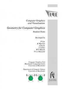
Figure 1: Our new data structure, the Inner Sphere Tree, is based on sphere packings in arbitrary polygonal objects (left). They are suitable for different kinds of geometric queries, namely proximity queries (middle) and the penetration volume (right).

Abstract

The progress of visual and aural sensations, thanks to the development of more powerful hardware in conjunction with improved algorithms, has revolutionized the immersion of modern computer games.

Based on our new geometric data structure, the inner sphere trees, we present fast and stable algorithms for different kinds of collision detection queries between rigid objects at haptic rates. Namely, proximity queries and the penetration volume, which is related to the water displacement of the overlapping region and thus corresponds to a physically motivated force.

Since the visual feedback and effects of today’s games have become extremely mature, it will be more and more important for games to provide realistic feedback to other senses, such as our haptic sense. On the hardware side, this has become possible in recent years by the advent of first inexpensive haptic devices on the consumer market, such as the Falcon from Novint. Research on force-feedback devices and algorithms has been done over 10 years, and has only fairly recently been introduced to games.1

The latter allows us to define a novel penalty-based collision response scheme that provides continuous forces and torques which are applicable to physically-based simulations as well as to haptic rendering scenarios. Moreover, we present a time-critical version of the penetration volume computation that is able to achieve very tight bounds within a fixed budget of query time.

However, while there is a large body of research on how to render forces given a collision and its contact information, the computation of the latter for massive models is still a challenge. First of all, this is due to the much higher effort to compute contact information. Second, this is due to the update rates that are necessary for haptic rendering, which need to be much higher than for visual rendering, i.e., 250–1000 Hz. And third, defining the contact information such that continuous contact forces can be derived is not always obvious.

The main idea of our new data structure is to bound the object from the inside with a set of non-overlapping bounding volumes. The results show performance at haptic rates both for proximity and penetration volume queries, independent from the polygon count of the objects. CR Categories: I.3.5 [Computing Methodologies]: Computational Geometry and Object Modeling—Geometric algorithms, Object hierarchies; I.3.7 [Computing Methodologies]: ThreeDimensional Graphics and Realism—Animation, Virtual reality

Therefore, one of the major challenges in haptic rendering for games is the computation of continuous forces at haptic rates. A solution to this challenge can also be utilized to do physically-based simulation of rigid bodies, which has become increasingly popular in games over the past few years.

Keywords: physically-based simulation, collision detection, haptic rendering, collision response

In this paper, we take advantage of the fact that in rendering haptic forces, as well as in most real-time applications that involve physically-based simulation, an absolutely correct determination of the forces acting on the virtual objects is not necessary.

1

Introduction

1.1

Main Contributions

∗ e-mail:

[email protected] † e-mail:[email protected]

Based on our new data structure, the Inner Sphere Trees (IST), we present the following novel ideas: - new contact information for stable penalty forces, i.e. the penetration volume; 1

This is in analogy to Nintendo’s Wii, which is a transfer and adaptation of the research on novel, intuitive, unintrusive input devices over the past 15 years.

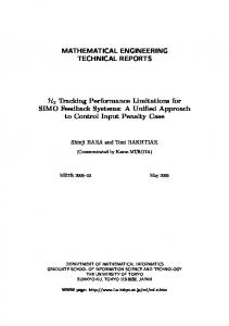
Figure 2: The different stages of our sphere packing algorithm: First, we voxelize the object (left) and compute distances from the voxels to the closest triangle (second image; transparency = distance). Then, we pick the voxel with the largest distance and put a sphere at its center. We proceed incrementally and, eventually, we obtain a dense sphere packing of the object (right).

- a unified algorithm that can compute both an approximate minimal distance and the approximate penetration volume for a pair of rigid objects; i.e., the application does not need to know in advance which situation currently exists between the pair of objects; - a time-critical variant of the penetration volume calculation, which runs only for a pre-defined time budget, including a new heuristic to derive good error bounds, the expected overlap volume; - a novel collision response scheme to compute stable and continuous forces and torques based on the penetration volume. The main idea of the ISTs is that we do not build an (outer) hierarchy based on the polygons on the boundary of an object, like most other BVHs do, but we fill the interior of the model with a set of non-overlapping simple volumes that cover the object’s volume densely. We used spheres in our implementation because of their convenient properties, but the idea of using inner BVs for lower bounds instead of outer BVs for upper bounds can be extended analogously to other kinds of volumes. On top of these inner BVs, we create a hierarchy in order to accelerate the computation of the approximate proximity and penetration volume queries. The penetration volume corresponds to the amount of water being displaced by the overlapping parts of the objects and, thus, leads to a physically motivated and continuous penalty force. According to [Fisher and Lin 2001, Sec. 5.1], it is “the most complicated yet accurate method” to define the extent of intersection, which was also reported earlier by [O’Brien and Hodgins 1999, Sec. 3.3]. However, to our knowledge, there are no algorithms to compute it efficiently as yet. Our data structure supports all kinds of object representations, e.g. polygon meshes or NURBS surfaces. They only have to be watertight. The construction of the ISTs consists of two main steps. First, we have to fill the object densely with a set of non-overlapping spheres. Therefore, we extended a flood filling voxelization algorithm and combined it with a special sphere creation scheme. The second step is to build a hierarchy upon these inner spheres for which we use a clustering approach. We describe the algorithm to compute both approximative separation distance and penetration volume based on the ISTs. In addition, we include improvements of the algorithm in quality and speed. The results show that our new data structure can answer both kinds of queries at haptic rates with a negligible loss of accuracy.

2

Previous Work

Collision detection has been extensively investigated by researchers in the past decades. There exist a large variety of freely available libraries for collision detection queries (see e.g. [Trenkel et al. 2007]). However, the number of libraries that also support the computation of proximity queries or the penetration depth is manageable. Additionally, most of them are not designed to work at haptic refresh rates. In the following, we will give a short overview of classical and also state of the art approaches.

2.1

BVH based data structures

In [Johnson and Cohen 1998] a generalized framework for minimum distance computations that depends on geometric reasoning and includes time-critical properties is presented. The PQP library [Larsen et al. 1999] uses swept sphere volumes as BVs in combination with several speed-up techniques for fast proximity queries. We used it in this paper to compute the ground truth for the proximity queries. Sphere trees have also been used for distance computation [Quinlan 1994; Hubbard 1995; Mendoza and O’Sullivan 2006]. The algorithms presented there are interruptible and they are able to deliver approximative distances. Moreover, they all compute a lower bound on the distance, while our ISTs derive an upper bound. Thus, a combination of these approaches with our ISTs could deliver error bounds in both directions. A local minimum distances for a stable force feedback computation is proposed by [Johnson and Willemsen 2003]. They use spatialized normal cone pruning for the collision detection. Another classical algorithm for proximity queries is the GJK [Gilbert et al. 1988; van den Bergen 1999], which computes the distance between a pair of convex objects, by utilizing the Minkowski sum of the two objects. Extensions to the GJK algorithms also allow to measure the penetration depth [Cameron 1997]. [Zhang et al. 2007] presented an extended definition of the penetration depth that also takes the rotational component into account, called the generalized penetration depth. However, this approach is computationally very expensive and, thus, might currently not be fast enough for haptic interaction rates. [Redon and Lin 2006] approximate a local penetration depth by first computing a local penetration direction and then use this information to estimate a local penetration depth on the GPU. Other GPU approaches have been presented by [Kim et al. 2003; Kim et al. 2002; Hoff et al. 2002] that also support proximity queries in image resolution. There is very little literature on penetration volume computation. [Hasegawa and Sato 2004] explicitly construct the intersection volume of convex polyhedra and apply this method to 6-DOF haptic rendering. However, this method is applicable only to very simple

geometries. Another approach mentioned by [Faure et al. 2008] computes an approximation of the intersection volume from layered depth images on the GPU. While this approach is applicable to deformable geometries, it is restricted to image space precision.

2.2

Voxel based data structures

Most 6-DOF haptic rendering approaches use the Voxmap Pointshell method [McNeely et al. 1999]. The main idea is to divide the virtual environment into a dynamic object, that is allowed to move freely through the virtual space and static objects that are fixed in the world. The static environment is discretized into a set of voxels, whereas the dynamic object is described by a set of points that represents its surface. During query time, for each of these points it is determined with a simple boolean test, whether it is located in a filled volume element or not. [Renz et al. 2001] presented extensions to the classic VPS, including optimizations to force calculation in order to increase its stability. However, even these optimizations cannot completely avoid the limits of VPS, namely aliasing effects, the huge memory consumption and the strict disjunction between dynamic and static objects. Closely related to VPS are distance field based methods. [Barbiˇc and James 2008] generates continuous contact forces for 6-DOF haptic rendering by using a pointshell of reduced deformable models in combination with distance fields.

3

Construction of the Inner Sphere Tree

In this section we describe the construction of our data structure. The goal is to fill an arbitrary object densely with a set of disjoint (i.e. non-overlapping) spheres such that the volume of the object is covered well while the number of spheres is as small as possible. In a second step, we build a hierarchy over this set of spheres. We chose spheres for volumes, because they offer a trivial and very fast overlap test. Moreover, they are rotationally invariant, and it is easy, in contrast to AABBs or OBBs, to compute the exact intersection volume.

3.1

Let there be Spheres

Filling objects densely with spheres is a highly non-trivial task. Bin packing, even when restricted to spheres, is still a very active field in geometric optimization and far away from being solved for general objects [Birgin and Sobral 2008; Schuermann 2006]. In our implementation of the inner sphere trees, we use a simple heuristic based on discrete distance field that offers a good trade-off between accuracy and speed in practice. Currently, we voxelize the object as an intermediate step (by a simple flood filling algorithm). But instead of only storing whether or not a voxel is filled, we additionally store the distance d from the center of the voxel to the nearest point on the surface. After the voxelization, we generate the inner spheres greedily. We choose the voxel V ∗ with the largest distance d∗ to the surface. We create an inner sphere with radius d∗ and centered on the center of V ∗ . All voxels whose centers are contained in this sphere will not be considered any further. Additionally, we have to update all voxels Vi within a radius 2d∗ around V ∗ and distance d(Vi , V ∗ ) < di + d∗ ; their di must now be set to the new free radius. This is, because they are now closer to the sphere around V ∗ than to a triangle on the hull. This process stops, when there is no voxel left. After these steps, the object is filled densely with a set of nonoverlapping spheres. The density can be controlled by the number

of voxels.

3.2

Building the Hierarchy

Based on the sphere packing, we create a bounding volume hierarchy. To do so, we use a top-down wrapped hierarchy approach, according to the notion of [Agarwal et al. 2004], where inner nodes are tight BVs for all their leaves, but they do not necessarily bound their direct children. We start with a bounding sphere for all inner spheres, which becomes the root node of the hierarchy. To compute that, we use the fast and stable smallest enclosing sphere algorithm proposed in [G¨artner 1999]. Then, we recursively divide the set of inner spheres into subsets in order to create the children. The partitioning of the spheres can be done by using any effective technique. In our examples, we use an approach based on a clustering algorithm called batch neural gas with magnification control (see [Hammer et al. 2006; Weller and Zachmann 2009] for details). Experiments with our data structure have shown that a branching factor of 4 produces the best results. Additionally, this has the benefit that we can use the full capacity of SIMD units in modern CPUs. In the following, we will call those spheres in the hierarchy that are not leaves hierarchy spheres. Spheres at the leaves, which were created in Section 3.1, will be called inner spheres. Note that hierarchy spheres are not necessarily contained completely within the object.

4

BVH Traversal

Our algorithm(s) for answering proximity queries and for computing the penetration volume work similarly to the classic recursive schemes that simultaneously traverse two given hierarchies [Zachmann 1998]. As a by-product, our algorithm can return a witness realizing the separation distance in the case of non-collision, and a partial list of intersecting polygons in the case of a penetration. In the following, we describe algorithms for these two query types, but it should be obvious how they can be modified in order to provide an approximate yes-no answer. This would further increase the speed. First, we will discuss the two query types separately, in order to point out their specific requirements and optimizations. Then, we explain how they can be combined into a single algorithm.

4.1

Proximity Queries

Our algorithm for proximity queries works like most other classical BVH traversal algorithms. We simply have to maintain, in addition, a lower bound for the distance. If a pair of leaves, which are inner spheres, is reached, we update the lower bound so far (see Algorithm 1). During traversal, there is no need to visit branches of the bounding volume test tree that are farther apart than the current minimum distance, because of the bounding property. This guarantees a high culling efficiency. 4.1.1

Improving runtime

In most collision detection scenarios, there is a high spatial and temporal coherence, especially when rendering at haptic rates. Thus, in most cases, those spheres realizing the minimum distance in a frame are also the closest spheres in the next frames, or they are at least in the neighborhood. Therefore, using the distance from the last frame yields a good initial bound for pruning during traversal. Thus, in our implementation we store pointers to the closest spheres as of

Algorithm 1: checkDistance( A, B, minDist ) input : A, B = spheres in the inner sphere tree in/out : minDist = overall minimum distance seen so far if A and B are leaves then // end of recursion

minDist = min{distance(A, B), minDist} else // recursion step

forall children a[i] of A do forall children b[j] of B do if distance(a[i], b[j]) < minDist then checkDistance( a[i], b[j], minDist )

Figure 4: We estimate the real penetration volume (brown) during our time-critical traversal by the “density” in the hierarchy spheres (green and red) and the total volume of the leaf spheres. Algorithm 2: computeVolume( A, B, totalOverlap ) input : A, B = spheres in the inner sphere tree in/out : totalOverlap = overall volume of intersection if A and B are leaves then // end of recursion

totalOverlap += overlapVolume( A, B ) else // recursion step

Figure 3: After constructing the sphere packing (see Section 3.1), every voxel can be intersected by several non-overlapping spheres (left). These do not necessarily account for the whole voxel space (blue space in the left picture). In order to account for these voids, too, we simply increase the radius of the sphere (blue sphere) that covers the center of the voxel (right).

the last frame and use their current distance to initialize minDist in Algorithm 1. If the application is only interested in the distance between a pair of objects, then, of course, a further speed-up can be gained by abandoning the traversal once the first pair of intersecting inner spheres is found (in this case the objects must overlap). Moreover, our traversal algorithm is very well suited for parallelization. During recursion, we compute the distances between 4 pairs of spheres in one single SIMD implementation, which is greatly facilitated by our hierarchy being a 4-ary tree. 4.1.2

Improving accuracy

forall children a[i] of A do forall children b[j] of B do if overlap(a[i], b[j]) > 0 then computeVolume( a[i], b[j], totalOverlap )

4.2.1

Filling the gaps

The algorithm described in Section 3.1 results in densely filled objects. However, there still remain small voids between the spheres that cannot be completely compensated by increasing the number of voxels. As a remedy, we assign an additional, secondary radius to each inner sphere, such that the volume of the secondary sphere is equal to the volume of all voxels whose centers are contained within the radius of the primary sphere.This guarantees that the total volume of all secondary spheres equals the volume of the object, within the accuracy of the voxelization, because each voxel volume is accounted for exactly once.

Obviously, Algorithm 1 returns only an approximate minimum distance, because it utilizes only the distances of the inner spheres for the proximity query. Thus, the accuracy depends on their density.

Certainly, these secondary spheres may slightly overlap, but this simple heuristic leads to acceptable estimations of the penetration volume.

Fortunately, it is very easy to alleviate these inaccuracies by simply assigning the closest triangle (or a set of triangles) to each inner sphere. After determining the closest spheres with Algorithm 1, we add a subsequent test that calculates the exact distance between the triangles assigned to those spheres. This simple heuristic reduces the error significantly even with relatively sparsely filled objects, and it does not affect the running time (see Figure 8).

4.2.2

4.2

Penetration Volume Queries

In addition to proximity queries, our data structure also supports a new kind of penetration query, namely the penetration volume. This is the volume of the intersection of the two objects, which can be interpreted directly as the amount of the repulsion force, if it is considered as the amount of water being displaced. Obviously, the algorithm to compute the penetration volume (see Algorithm 2) does not differ very much from the proximity query test: we simply have to replace the distance test by an overlap test and maintain an accumulated overlap volume during the traversal.

Improvements

Similar to the proximity query implementation, we can utilize SIMD parallelization to speed up both the simple overlap check and the volume accumulation. Furthermore, we can exploit the observation that a recursion can be terminated if a hierarchy sphere (i.e., an inner node of the sphere hierarchy) is completely contained inside an inner sphere (leaf)of the other IST. In this case, we can simply add the total volume of all of its leaves to the accumulated penetration volume. In order to do this quickly, we store the total volume Voll (S) =

X

Vol(Sj ),

(1)

Sj ∈Leaves(S)

where Sj are all inner spheres below S in the BVH. This can be done in a preprocessing step during hierarchy creation.

Algorithm 3: compVolumeTimeCritical( A, B ) input : A, B = root spheres of the two ISTs estOverlap = Vol(A, B) Q = empty priority queue Q.push( A, B ) while Q not empty & time not exceeded do (R, S) = Q.pop() if R and S are not leaves then estOverlap –= Vol(R, S) forall Ri ∈ children of R, Sj ∈ children of S do estOverlap += Vol(Ri , Sj ) Q.push( Ri , Sj )

volume Vol(R, S) as the probability that a point is inside R ∩ S and also inside the intersection of one of the possible pairs of leaves, i.e., Vol(R, S) = p(S) · p(R) · Vol(R ∩ S) =

Voll (R) · Voll (S) · Vol(R ∩ S) Vol(R) · Vol(S)

(4)

(see Figure 4). In summary, for the whole queue we get the expected overlap volume X Vol(R, S) (5) (R,S)∈Q

Clearly, this volume can be maintained during traversal quite easily. 4.2.3

Time-critical computation of penetration volume

In most cases, a penetration volume query has to visit many more nodes than the average proximity query. Consequently, the running time on average is slower, especially in cases with heavy overlaps. In the following, we will describe a variation of our algorithm for penetration volume queries that guarantees a predefined query time budget. This is essential for time-critical applications such as haptic rendering. A suitable strategy to realize time-critical traversals is to guide the traversal by a priority queue Q. Then, given a pair of hierarchy spheres S and R, a simple heuristic is to use Vol(S ∩ R) for the priority in Q. In our experience, this would yield acceptable upper bounds. Unfortunately, this simple heuristic also leads to very bad lower bounds in cases where only a relatively small number of inner spheres can be visited (unless the time budget permits an almost complete traversal of all overlapping pairs). A simple heuristic to derive an estimate of the lower bound could be to compute X X Vol(Ri ∩ Sj ), (2) (R,S)∈Q Ri ∈ch(R), Sj ∈ch(S)

where ch(S) is the set of all direct children of node S. Equation 2 amounts to the sum of the intersection of all direct child pairs of all pairs in the p-queue Q. Unfortunately, the direct children of a node are usually not disjoint and, thus, this estimate of the lower bound could actually be larger than the upper bound. In order to avoid this problem, we introduce the notion of expected overlap volume in order to estimate the overlap volume more accurately. The only assumption we make is that for any point inside S, the distribution of the probability that it is also inside one of its leaves is uniform. Let (R, S) be a pair of spheres in the p-queue. We define the density of a sphere as Voll (S) (3) p(S) = Vol(S) with voll (S) defined similarly to equation 1 as the accumulated volume of all inner spheres below S. This is the probability that a point inside S is also inside one of its leaves (which are disjoint). Next, we define the expected overlap

More importantly, this method provides a much better heuristic for sorting the priority queue: if the difference between the expected overlap Vol(R, S) and the overlap Vol(R ∩ S) is large, then it is most likely that the traversal of this pair will give the most benefit toward improving the bound; consequently, we insert this pair closer to the front of the queue. Algorithm 3 shows the pseudo code of this approach. (Note that p(S) = 1 if S is a leaf, and therefore Vol(R, S) returns the exact intersection volume at the leaves.)

4.3

The Unified Algorithm

In the previous sections, we introduced the proximity and the penetration volume computation separately. However, it is of course possible to combine both algorithms. This yields a unified algorithm that can compute both the distance and the penetration volume. To that end, we start with the distance traversal. As soon as we find the first pair of intersecting inner spheres, we simply switch to the penetration volume computation. This is correct because all pairs of inner spheres we visited so far did not overlap and thus they could not increase the penetration volume. Thus, we do not have to visit them again and can continue with the traversal of the rest of the hierarchies using the penetration volume algorithm. If we do not meet an intersecting pair of inner spheres, the unified algorithm still reports the minimal separating distance.

5

Collision Response

In this section, we describe how to use the penetration volume to compute continuous forces in order to enable a stable haptic rendering. Mainly, there exist three different approaches to resolve collisions: the penalty-based method, the constraint-based method and the impulse-based method. The constraint-based approach computes constraint forces that are designed to cancel any external acceleration that would result in interpenetrations. Unfortunately, this method has at least quadratic complexity in the number of contact points. The impulse-based method resolves contacts between objects by a series of impulses in order to prevent interpenetrations. It is applicable to real-time simulations but the forces may not be valid for bodies in resting contact. So, we decided to use the penalty-based method, that computes penalty forces based on the interpenetration of a pair of objects. The main advantages are its computational simplicity, which makes it applicable for haptic rendering, and its ability to simulate a variety of surface characteristics. Moreover, the use of the penetration

110

1 0.8

100

0.6 90

0.4 0.2

Magnitude Direction

0.3 Torque Magnitude

120

1.2

Force Direction in Deg

Magnitude Direction

1.4 Force Magnitude

Torque 0.35

130

80 0

100

200 300 Frame

400

80

0.2

70

0.15

60

0.1

50

0.05

40 0

500

90

0.25

0

0

100

100

200 300 Frame

400

Torque Direction in Deg

Force 1.6

30 500

Figure 6: Left: magnitude (red) and direction (blue) of the force arising between two copies of the object shown in the middle, one of which is being moved on a pre-recorded path. Right: torque magnitude (red) and direction (blue) in the same scene.

to compute normal cones, which are defined by an axis and an angle. They tightly bound the normals of the triangles that are stored in the list of each inner sphere.

cR

During force computation, the axes of the normal cones cR and cS are used as the directions of the force, since they will bring the penetrating spheres outside the other object in the direction of the surface normals (see Figure 5). Note that f (Ri ) 6= f (Sj ). If the cone angle is too large (i.e., α ≈ π), then we simply use the vector between the two centers of the spheres.

PR,S cS Figure 5: Left: We compute a normal cone for each inner sphere. The cone bounds a list of triangles that is associated with the sphere. Note that the spread angle of the normal cone can be 0 if the sphere is closest to a single triangle (e.g., the green sphere). Right: The axis of the normal cones cR and cS are used for the force direction. The center PR,S of the spherical cap defines the contact point.

volume eliminates inconsistent states that may occur when only a penetration depth (e.g. a minimum translational vector) is used.

5.1

Contact Forces

Algorithm 2, and its time-critical derivative, return a set of overlapping spheres or potentially overlapping spheres, resp. We compute a force for each of these pairs of spheres (Ri , Sj ) by: f (Ri ) = kc Vol(Ri ∩ Sj )n(Ri )

(6)

where kc is the contact stiffness, Vol(Ri ∩ Sj ) is the overlap volume, and n(Ri ) is the contact normal. Summing up all pairwise forces gives the total penalty force: X f (R) = f (Ri )

Obviously, this force is continuous in both cases, because the movement of the axes of the normal cones and also the movement of the centers of the spheres are continuous, provided the path of the objects is continuous. See Figure 6 for results from our benchmark.

5.2

Torques

In rigid body simulation, the torque τ is usually computed as τ = (Pc −Cm )×f , where Pc is the point of collision, Cm is the center of mass of the object and f is the force acting at Pc . Like in the section before, we compute the torque separately for each pair (Ri , Sj ) of intersecting inner spheres: τ (Ri ) = (P(Ri ,Sj ) − Cm ) × f (Ri )

(8)

Again, we accumulate all pairwise torques to get the total torque: X τ (R) = τ (Ri ) (9) Ri ∩Sj 6=∅

We define the point of collision P(Ri ,Sj ) simply as the center of the intersection volume of the two spheres (see Figure 5). Obviously, this point moves continuously if the objects move continuously. In combination with the continuous forces f (Ri ) this results in a continuous torque.

6

Results

(7)

Ri ∩Sj 6=∅

In order to compute normals for each pair of spheres, we augment the construction process of the ISTs: in addition to storing the distance to the object’s surface, we store a pointer to the triangle that realizes this minimum distance. While creating the inner spheres by merging several voxels (Section 3.1), we accumulate a list of triangles for every inner sphere. We use the normals of these triangles

We have implemented our new data structure in C++ on a PC running Windows XP with an Intel Pentium IV 3GHz dual core CPU and 2GB of memory. We extended Dan Morris’ Voxelizer [Morris 2006] to compute the initial distance field. We used several hand recorded object paths for our benchmarks. For the proximity queries, we focused on very close configurations, within a distance range of about 0–10% of the object’s BV size, because these are most stressing and also more relevant to real world

scenarios than larger distances. The paths for the penetration volume tests concentrate on light to medium penetrations of about 0– 10% of the object’s volume, because this best resembles the usage in haptic applications and physically-based simulations. In addition, we included some heavy penetrations of 50% of the object’s volume to stress our algorithm. We used several different objects to test the performance of our algorithms with a polygon count ranging up to 700k triangles per object in the armadillo scene (see Figure 7). We voxelized each object in different resolutions in order to evaluate the trade-off between the number of spheres and the accuracy. This trade-off is independent of the object’s complexity but depends on the density of inner spheres.2 We used PQP to compute the exact distance and measure the quality of our distance approximation. The running time of PQP is not directly comparable to our ISTs because of the more time consuming exact distance computation. Thus, we did not include the timings in our plots. Just to give the reader a sense of the speed-up: our approximative approach is between 20–120 times faster than the exact PQP, depending on the density of the inner spheres. To our knowledge, there are no publicly available implementations to compute the penetration volume efficiently. In order to evaluate the quality of our penetration volume approximation, we used a tetrahedralization of the objects. The non-overlapping tetrahedra fill the objects without any gaps, and thus we can calculate the intersection volume exactly. Additionally, we build a hierarchy on top of the tetrahedra in order to accelerate penetration volume queries. However, the runtime of this approach is not applicable to real-time applications due to bad BV fitting and the costly tetrahedron-tetrahedron overlap volume calculation. It takes more than 2 sec/frame on average within all our scenarios. The results from our benchmark prove that the distance queries can be done at haptic rates even for very large objects with hundreds of thousands of polygons (see Figure 7). The approximation error is less than 1%. The accuracy can be further improved by the simple extension described in Section 4.1.2. With the highest sphere count, the error is below floating point accuracy with only a negligible longer running time (see Figure 8). Also, our penetration volume queries perform at haptic rates of at least 200 Hz on average (see Figure 9). Again, the error is considerably smaller than 1% when using an adequate amount of inner spheres. However, in the case of deeper penetrations, it is possible that the traversal algorithm may exceed its time budget for haptic rendering. In this case, our time-critical traversal guarantees acceptable estimations of the penetration volume even in worst-case scenarios and multiple contacts (see Figure 10).

7

Conclusions and Future Work

We have presented a novel hierarchical data structure, the inner sphere trees, that supports both proximity queries and penetration volume computations with one unified algorithm. Both kinds can be answered at rates of about 1 kHz (which makes the algorithm suitable for haptic rendering) even for very complex objects with several hundreds of thousands of polygons. For proximity situations, typical average runtimes are in the order of less than 0.5 msec with 500 000 spheres per object and an error of about 0.5%. Obviously, the running times depend much more on the intersection volume in penetration situations; here, we are in the 2

Please visit cg.in.tu-clausthal.de/research/ist/ to watch some videos of our benchmarks.

order of around 5 msec on average with 250 000 spheres and an error of about 0.7%. The balance between accuracy and speed can be specified by the user, and it is independent of the object complexity, because the number of leaves of our hierarchy is mostly independent of the number of polygons. For time-critical applications, we described a variant of our algorithm that stays within a fixed time budget while returning an answer “as good as possible”. Our algorithm for both kinds of queries can be integrated into existing simulation software very easily, because there is only a single entry point, i.e., the application does not need to know in advance whether or not a given pair of objects will be penetrating each other. Memory consumption of our inner sphere trees is similar to other sphere hierarchies, depending on the predefined accuracy (in our experiments, it was always in the order of a few MB). This is very modest compared to voxel-based approaches. Another big advantage of our penetration volume algorithm is that it yields a continuous measure for penetration and force direction as well as a stable heuristic for torque computations. Last but not least, inner sphere trees are perfectly suited for SIMD acceleration techniques and allow algorithms to make heavy use of temporal and spatial coherence. Our novel approach opens up several avenues for future work. First of all, we are currently working on replacing the intermediate distance field by a Voronoi-based approach to generate better sphere packings. This is a challenging task, because several goals should be met: accuracy, query efficiency, and small build times. We are confident that this will also result in analytically predictable error bounds. Furthermore, a GPU implementation of the force computation should result in further speed-ups. This is possible, because the forces and torques depend only on computations on a set of independent pairs of spheres, which is (almost) trivially parallelizable. Another option could be the investigation of inner volumes other than spheres. This could improve the quality of the volume covering, because spheres do not fit well into some objects, especially if they have many sharp corners or thin ridges. Until now, our approach is restricted to watertight objects. In the future, we plan to extend the ISTs so that they are also able to handle arbitrary objects, including thin sheets and open geometries. Finally, a challenging task would be to extend our approach also to deformable objects.

Acknowledgment This work was partially supported by DFG grant ZA292/1-1 and BMBF grant Avilus / 01 IM 08 001 U.

References AGARWAL , G UIBAS , N GUYEN , RUSSEL , AND Z HANG. 2004. Collision detection for deforming necklaces. CGTA: Computational Geometry: Theory and Applications 28. BARBI Cˇ , J., AND JAMES , D. L. 2008. Six-dof haptic rendering of contact between geometrically complex reduced deformable models. IEEE Transactions on Haptics 1, 1, 39–52. B IRGIN , E. G., AND S OBRAL , F. N. C. 2008. Minimizing the object dimensions in circle and sphere packing problems. Computers & OR 35, 7, 2357–2375.

14

2.5

12

2 1.5 1

Error in %

0.7 0.6 0.5 0.4 0.3 0.2 0.1 0

Distance Error 3

msec

msec

Running Time (Avg Max) IST (5 k) IST (35 k) IST (185 k) IST (508 k)

10

IST (5 k) IST (35 k) IST (185 k) IST (508 k)

8 6 4

0.5

2

0

0

Figure 7: Left: snapshot of distance computation in the armadillo scene (700k triangles) Center: average and maximum query time; note the two different y axes: the left one is for the average running times, the right one for the maximum times. Right: relative error compared to exact distance.

Average Running Time 0.5 msec

0.4 0.3

Distance Error 12

IST (4 k) IST (27 k) IST (157 k) IST (446 k) IST (4 k) IA IST (27 k) IA IST (157 k) IA IST (446 k) IA

IST (4 k) IST (27 k) IST (157 k) IST (446 k) IST (4 k) IA IST (27 k) IA IST (157 k) IA IST (446 k) IA

10 Error in %

0.6

0.2

8 6 4

0.1

2

0

0

Figure 8: Improvement of the accuracy (IA, right group of measurement) described in Section 4.1.2. Left: average running time. Center: error compared to exact distance. Right: snapshot of the scenario.

Running Time (Avg Max)

Volume Error 30

12

25

10

4

20

3

15

2

10

1

5

2

0

0

0

msec

msec

5

IST (2 k) IST (16 k) IST (89 k) IST (249 k)

Error in %

6

IST (2 k) IST (16 k) IST (89 k) IST (249 k)

8 6 4

Figure 9: Right: snapshot from the screwdriver scene that we used for penetration volume computation (488k triangles). Center: average and maximum query time; note the two different y axes. Right: relative error compared to exact volume.

Running Time (Avg Max)

msec

5 4 3 2 1 0

Error of Time Critical Traversal 40 35 30 25 20 15 10 5 0

Error in %

6

IST (2 k) IST (14 k) IST (83 k) IST (228 k)

msec

7

80 70 60 50 40 30 20 10 0 -10

(228 k)

0 50 100 150 200 250 300 Number of Sphere/Sphere Tests / 1000

Figure 10: Time critical penetration volume computations in the torso scene (470k triangles). Left: average and maximum query time; again, the y axes are labeled different. Center: error relative to the exact penetration volume depending on the number of intersection tests. Right: snapshot.

C AMERON , S. 1997. Enhancing GJK: Computing minimum and penetration distances between convex polyhedra. In Proceedings of International Conference on Robotics and Automation, 3112– 3117. FAURE , F., BARBIER , S., A LLARD , J., AND FALIPOU , F. 2008. Image-based collision detection and response between arbitrary volumetric objects. In ACM Siggraph/Eurographics Symposium on Computer Animation, SCA 2008, July, 2008. F ISHER , S. M., AND L IN , M. C., 2001. Fast penetration depth estimation for elastic bodies using deformed distance fields.

M ENDOZA , C., AND O’S ULLIVAN , C. 2006. Interruptible collision detection for deformable objects. Computers & Graphics 30, 3, 432–438. M ORRIS , D. 2006. Algorithms and data structures for haptic rendering: Curve constraints, distance maps, and data logging. In Technical Report 2006-06. O’B RIEN , J. F., AND H ODGINS , J. K. 1999. Graphical modeling and animation of brittle fracture. In SIGGRAPH ’99: Proceedings of the 26th annual conference on Computer graphics and interactive techniques, ACM Press/Addison-Wesley Publishing Co., New York, NY, USA, 137–146.

¨ G ARTNER , B. 1999. Fast and robust smallest enclosing balls. In ESA, Springer, J. Nesetril, Ed., vol. 1643 of Lecture Notes in Computer Science, 325–338.

Q UINLAN , S. 1994. Efficient distance computation between nonconvex objects. In In Proceedings of International Conference on Robotics and Automation, 3324–3329.

G ILBERT, E. G., J OHNSON , D. W., AND K EERTHI , S. S. 1988. A fast procedure for computing the distance between complex objects in three-dimensional space. IEEE Journal of Robotics and Automation 4, 193–203.

R EDON , S., AND L IN , M. C. 2006. A fast method for local penetration depth computation. Journal of Graphics Tools: JGT 11, 2, 37–50.

H AMMER , B., H ASENFUSS , A., AND V ILLMANN , T. 2006. Magnification control for batch neural gas. In ESANN, 7–12. H ASEGAWA , S., AND S ATO , M. 2004. Real-time rigid body simulation for haptic interactions based on contact volume of polygonal objects. Comput. Graph. Forum 23, 3, 529–538. H OFF , K. E., Z AFERAKIS , A., L IN , M., AND M ANOCHA , D. 2002. Fast 3d geometric proximity queries between rigid & deformable models using graphics hardware acceleration. Tech. Rep. TR02-004, Department of Computer Science, University of North Carolina - Chapel Hill, Mar. 7. Fri, 8 Mar 2002 20:06:33 GMT.

R ENZ , M., P REUSCHE , C., P TKE , M., PETER K RIEGEL , H., AND H IRZINGER , G. 2001. Stable haptic interaction with virtual environments using an adapted voxmap-pointshell algorithm. In In Proc. Eurohaptics, 149–154. S CHUERMANN , A. 2006. On packing spheres into containers (about Kepler’s finite sphere packing problem). In Documenta Mathematica, vol. 11, 393–406. T RENKEL , S., W ELLER , R., AND Z ACHMANN , G. 2007. A benchmarking suite for static collision detection algorithms. In International Conference in Central Europe on Computer Graphics, Visualization and Computer Vision (WSCG), Union Agency, Plzen, Czech Republic, V. Skala, Ed. B ERGEN , G. 1999. A fast and robust GJK implementation for collision detection of convex objects. Journal of Graphics Tools: JGT 4, 2, 7–25.

VAN DEN

H UBBARD , P. M. 1995. Collision detection for interactive graphics applications. IEEE Transactions on Visualization and Computer Graphics 1, 3 (Sept.), 218–230. J OHNSON , D. E., AND C OHEN , E. 1998. A framework for efficient minimum distance computations. In Proceedings of the IEEE International Conference on Robotics and Automation (ICRA98), IEEE Computer Society, Piscataway, 3678–3684. J OHNSON , D. E., AND W ILLEMSEN , P. 2003. Six degree-offreedom haptic rendering of complex polygonal model. In HAPTICS, IEEE Computer Society, 229–235. K IM , Y., OTADUY, M., L IN , M., AND M ANOCHA , D. 2002. Fast penetration depth computation for physically-based animation. In Proceedings of the 2002 ACM SIGGRAPH Symposium on Computer Animation (SCA-02), ACM Press, New York, S. N. Spencer, Ed., 23–32. K IM , OTADUY, L IN , AND M ANOCHA. 2003. Fast penetration depth estimation using rasterization hardware and hierarchical refinement (short). In COMPGEOM: Annual ACM Symposium on Computational Geometry. L ARSEN , E., G OTTSCHALK , S., L IN , M., AND M ANOCHA , D. 1999. Fast proximity queries with swept sphere volumes. In Technical Report TR99-018. M C N EELY, W. A., P UTERBAUGH , K. D., AND T ROY, J. J. 1999. Six degrees-of-freedom haptic rendering using voxel sampling. In Siggraph 1999, Addison Wesley Longman, Los Angeles, A. Rockwood, Ed., Annual Conference Series, ACM Siggraph, 401–408.

W ELLER , R., AND Z ACHMANN , G. 2009. Inner sphere trees for proximity and penetration queries. In Robotics: Science and Systems (RSS). Z ACHMANN , G. 1998. Rapid collision detection by dynamically aligned DOP-trees. In Proc. of IEEE Virtual Reality Annual International Symposium; VRAIS ’98, 90–97. Z HANG , L., K IM , Y. J., VARADHAN , G., AND M ANOCHA , D. 2007. Generalized penetration depth computation. ComputerAided Design 39, 8, 625–638.