Computer Graphics

Computer Science Aston University Birmingham B4 7ET http://www.cs.aston.ac.uk/

Computer Graphics Dan Cornford CS2150

1

September 20, 2004

Course Outline

OUTPUT

INPUT

Image

Description

Image

Image Processing

Pattern Recognition

Description

Computer Graphics

Data Processing

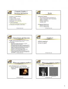
This course is meant as an introduction to computer graphics, which covers a large body of work. The intention is to give a solid grounding in basic 2D computer graphics and introduce the concepts and some techniques required to implement 3D graphics. In order to achieve as complete an understanding as possible, we investigate the low level methods used in computer graphics while using OpenGL, a high level computer graphics Application Programmer Interface (API) to code up and use many of the methods discussed. Image processing is also briefly introduced, but in a more descriptive manner in the last part of the course.

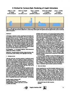
Figure 1.1: What is computer graphics?

Computer graphics sits at the interface between the Image and the Description (of that image) as shown in Figure 1.1. The most simple explanation of computer graphics, is the complete processes of taking a Description of an object or scene, and producing an Image of that object or scene using a computer. Image processing, on the other hand takes in an Image and alters it in some way to produce another Image. Note that this module embraces the left hand column, the right hand column being essentially the concern of statistics and pattern recognition.

1.1

Course philosophy

The course is loosely based on Foley et al. (1993) and thus this is the recommended reading for the course, although most will probably find an OpenGL book more useful. The first part of the course will concentrate on the knowledge necessary to understand computer graphics using methods and algorithms for 2D graphics as examples. The second part develops the concepts into the 3D graphics domain with an introduction to some of the methods used to generate realistic representations of real world objects. In the third part of the module the hardware background and some related algorithms are reviewed. In the final part of the course a brief introduction to image processing and associated techniques is given. This should give you both a solid foundation in computer graphics and an appreciation of the breadth and complexity of the modern subject. The lab classes introduce some standard programming approaches to computer graphics, using OpenGL. OpenGL is probably the most widely used cross platform graphics API. Although Direct 3D (written by Microsoft) is also very popular on PC systems, OpenGL has the advantage of being supported on almost all platforms, with bindings to almost all of the commonly used languages. Thus the lab classes support the lecturing material, often implementing what is covered in the lectures. We will use C in the labs, and thus the first few labs will involve teaching you basic C. I will not spend too much time on this, however, since this is not a programming module. Note that the syntax of C is almost identical to Java, so you are not being made to learn a completely new language.

2

CS2150 Computer Graphics

1.2

Course composition

The course consists of the following main sections: ➢ ➢ ➢ ➢ ➢ ➢ ➢ ➢ ➢ ➢

1.3

why study computer graphics; 2D geometrical transformations and clipping; 3D computer graphics; curves and surfaces. visible surface problem, illumination and shading; conceptual models for computer graphics; computer graphics hardware issues; raster algorithms for 2D computer graphics; image formats and compression; image processing.

Recommended reading

These lecture notes contain enough detail to pass the CS215 exam, however to get a good grade you will need to attend the lectures and practicals and do some independent reading. There are two good books which cover almost all the material in the course: Foley et al. (1993) and Hearn and Baker (1994). There is really very little to choose between them - of the two Hearn and Baker (1994) has a little more mathematics - although really they are very similar in content. Neither book covers OpenGL which is used in the lab classes, so an alternative might be Hill (2000), however this book is rather difficult to read and uses rather a lot of C++– check it out before you buy it. If you are really interested in computer graphics and you have funds available then Foley et al. (1996) is a very complete volume covering all aspects of computer graphics, and will serve as a useful future reference. If you are more interested in the programming side and want to learn more about OpenGL, then Woo et al. (1999) is a very well written book, if a little expensive. A cheaper alternative is Angel (2002) which is cheaper, and covers quite a bit of OpenGL, but no graphics theory. The library has copies of all the above books, and many more (check out the class-marks 006.6 in the library). Short loan should hold at least one copy of the key books. The library also takes a number of journals which cover computer graphics matters, on the first floor.

References Angel, E. 2002. OpenGL: A primer. London: Addison-Wesley. Foley, J., A. van Dam, S. K. Feiner, and J. F. Hughes 1996. Computer Graphics: Principles and Practice (Second Edition in C ed.). Reading, Massachusetts: Addison-Wesley. Foley, J., A. van Dam, S. K. Feiner, J. F. Hughes, and R. L. Phillips 1993. Introduction to Computer Graphics. Reading, Massachusetts: Addison-Wesley. Hearn, D. and P. M. Baker 1994. Computer Graphics (Second Edition ed.). London: Prentice Hall. Hill, F. S. 2000. Computer Graphics using OpenGL (Second Edition ed.). London: Prentice Hall. Woo, M., J. Neider, T. Davis, and D. Shreiner 1999. OpenGL Programming Guide (Third Edition ed.). Reading, Massachusetts: Addison-Wesley.


3

Contents 1 Course Outline

1

1.1

Course philosophy . . . . . . . . . . . . . . . . . . . . . . . . . . . . . . . . . . . . . . . . . . . . . . . . . . . . . . . . . . . . . . . . . . . . . . . . . . . . . . . . . . . . . . . . . . . . . . . . . . .

1

1.2

Course composition . . . . . . . . . . . . . . . . . . . . . . . . . . . . . . . . . . . . . . . . . . . . . . . . . . . . . . . . . . . . . . . . . . . . . . . . . . . . . . . . . . . . . . . . . . . . . . . . . .

2

1.3

Recommended reading . . . . . . . . . . . . . . . . . . . . . . . . . . . . . . . . . . . . . . . . . . . . . . . . . . . . . . . . . . . . . . . . . . . . . . . . . . . . . . . . . . . . . . . . . . . . . .

2

2 Why Study Computer Graphics? 2.1

A very brief history . . . . . . . . . . . . . . . . . . . . . . . . . . . . . . . . . . . . . . . . . . . . . . . . . . . . . . . . . . . . . . . . . . . . . . . . . . . . . . . . . . . . . . . . . . . . . . . . .

3 2D Geometrical Transformations

6 6 7

3.1

Vectors . . . . . . . . . . . . . . . . . . . . . . . . . . . . . . . . . . . . . . . . . . . . . . . . . . . . . . . . . . . . . . . . . . . . . . . . . . . . . . . . . . . . . . . . . . . . . . . . . . . . . . . . . . . . . . .

7

3.2

Matrices . . . . . . . . . . . . . . . . . . . . . . . . . . . . . . . . . . . . . . . . . . . . . . . . . . . . . . . . . . . . . . . . . . . . . . . . . . . . . . . . . . . . . . . . . . . . . . . . . . . . . . . . . . . . . .

8

3.3

2D transformations . . . . . . . . . . . . . . . . . . . . . . . . . . . . . . . . . . . . . . . . . . . . . . . . . . . . . . . . . . . . . . . . . . . . . . . . . . . . . . . . . . . . . . . . . . . . . . . . . .

9 9

3.4

Homogeneous coordinates . . . . . . . . . . . . . . . . . . . . . . . . . . . . . . . . . . . . . . . . . . . . . . . . . . . . . . . . . . . . . . . . . . . . . . . . . . . . . . . . . . . . . . . . . . .

3.5

Composition of transformations . . . . . . . . . . . . . . . . . . . . . . . . . . . . . . . . . . . . . . . . . . . . . . . . . . . . . . . . . . . . . . . . . . . . . . . . . . . . . . . . . . . . 10

3.6

Window to viewport transformation . . . . . . . . . . . . . . . . . . . . . . . . . . . . . . . . . . . . . . . . . . . . . . . . . . . . . . . . . . . . . . . . . . . . . . . . . . . . . . . 10 3.6.1 Efficiency . . . . . . . . . . . . . . . . . . . . . . . . . . . . . . . . . . . . . . . . . . . . . . . . . . . . . . . . . . . . . . . . . . . . . . . . . . . . . . . . . . . . . . . . . . . . . . . . . . . . . 12 3.6.2 Inverse transformations . . . . . . . . . . . . . . . . . . . . . . . . . . . . . . . . . . . . . . . . . . . . . . . . . . . . . . . . . . . . . . . . . . . . . . . . . . . . . . . . . . . . . 12

4 Viewing in 3D

13

4.1

Geometric modelling . . . . . . . . . . . . . . . . . . . . . . . . . . . . . . . . . . . . . . . . . . . . . . . . . . . . . . . . . . . . . . . . . . . . . . . . . . . . . . . . . . . . . . . . . . . . . . . . 13

4.2

3D coordinate systems . . . . . . . . . . . . . . . . . . . . . . . . . . . . . . . . . . . . . . . . . . . . . . . . . . . . . . . . . . . . . . . . . . . . . . . . . . . . . . . . . . . . . . . . . . . . . . 14

4.3

Transformations in 3D . . . . . . . . . . . . . . . . . . . . . . . . . . . . . . . . . . . . . . . . . . . . . . . . . . . . . . . . . . . . . . . . . . . . . . . . . . . . . . . . . . . . . . . . . . . . . . 15

4.4

Transforming lines and planes . . . . . . . . . . . . . . . . . . . . . . . . . . . . . . . . . . . . . . . . . . . . . . . . . . . . . . . . . . . . . . . . . . . . . . . . . . . . . . . . . . . . . . 16

4.5

Transformations are a change of coordinate systems . . . . . . . . . . . . . . . . . . . . . . . . . . . . . . . . . . . . . . . . . . . . . . . . . . . . . . . . . . . . . 17

4.6

Projection . . . . . . . . . . . . . . . . . . . . . . . . . . . . . . . . . . . . . . . . . . . . . . . . . . . . . . . . . . . . . . . . . . . . . . . . . . . . . . . . . . . . . . . . . . . . . . . . . . . . . . . . . . . . 4.6.1 Perspective projections . . . . . . . . . . . . . . . . . . . . . . . . . . . . . . . . . . . . . . . . . . . . . . . . . . . . . . . . . . . . . . . . . . . . . . . . . . . . . . . . . . . . . 4.6.2 Parallel projections . . . . . . . . . . . . . . . . . . . . . . . . . . . . . . . . . . . . . . . . . . . . . . . . . . . . . . . . . . . . . . . . . . . . . . . . . . . . . . . . . . . . . . . . . . 4.6.3 Specification of 3D views . . . . . . . . . . . . . . . . . . . . . . . . . . . . . . . . . . . . . . . . . . . . . . . . . . . . . . . . . . . . . . . . . . . . . . . . . . . . . . . . . . .

18 19 20 20

4.7

Implementing 3D→2D projections . . . . . . . . . . . . . . . . . . . . . . . . . . . . . . . . . . . . . . . . . . . . . . . . . . . . . . . . . . . . . . . . . . . . . . . . . . . . . . . . . 4.7.1 Parallel projections . . . . . . . . . . . . . . . . . . . . . . . . . . . . . . . . . . . . . . . . . . . . . . . . . . . . . . . . . . . . . . . . . . . . . . . . . . . . . . . . . . . . . . . . . . 4.7.2 Perspective projections . . . . . . . . . . . . . . . . . . . . . . . . . . . . . . . . . . . . . . . . . . . . . . . . . . . . . . . . . . . . . . . . . . . . . . . . . . . . . . . . . . . . . 4.7.3 Clipping . . . . . . . . . . . . . . . . . . . . . . . . . . . . . . . . . . . . . . . . . . . . . . . . . . . . . . . . . . . . . . . . . . . . . . . . . . . . . . . . . . . . . . . . . . . . . . . . . . . . . . 4.7.4 Projection . . . . . . . . . . . . . . . . . . . . . . . . . . . . . . . . . . . . . . . . . . . . . . . . . . . . . . . . . . . . . . . . . . . . . . . . . . . . . . . . . . . . . . . . . . . . . . . . . . . . 4.7.5 Viewport transformation. . . . . . . . . . . . . . . . . . . . . . . . . . . . . . . . . . . . . . . . . . . . . . . . . . . . . . . . . . . . . . . . . . . . . . . . . . . . . . . . . . . . 4.7.6 Overview . . . . . . . . . . . . . . . . . . . . . . . . . . . . . . . . . . . . . . . . . . . . . . . . . . . . . . . . . . . . . . . . . . . . . . . . . . . . . . . . . . . . . . . . . . . . . . . . . . . . .

22 22 24 25 25 25 26

5 Surface Modelling

27

5.1

Polygonal Meshes . . . . . . . . . . . . . . . . . . . . . . . . . . . . . . . . . . . . . . . . . . . . . . . . . . . . . . . . . . . . . . . . . . . . . . . . . . . . . . . . . . . . . . . . . . . . . . . . . . . . 27

5.2

Solid modelling . . . . . . . . . . . . . . . . . . . . . . . . . . . . . . . . . . . . . . . . . . . . . . . . . . . . . . . . . . . . . . . . . . . . . . . . . . . . . . . . . . . . . . . . . . . . . . . . . . . . . . 5.2.1 Primitive instancing . . . . . . . . . . . . . . . . . . . . . . . . . . . . . . . . . . . . . . . . . . . . . . . . . . . . . . . . . . . . . . . . . . . . . . . . . . . . . . . . . . . . . . . . . 5.2.2 Sweep representations . . . . . . . . . . . . . . . . . . . . . . . . . . . . . . . . . . . . . . . . . . . . . . . . . . . . . . . . . . . . . . . . . . . . . . . . . . . . . . . . . . . . . . . 5.2.3 Boundary representations . . . . . . . . . . . . . . . . . . . . . . . . . . . . . . . . . . . . . . . . . . . . . . . . . . . . . . . . . . . . . . . . . . . . . . . . . . . . . . . . . . . 5.2.4 Spatial partitioning representations . . . . . . . . . . . . . . . . . . . . . . . . . . . . . . . . . . . . . . . . . . . . . . . . . . . . . . . . . . . . . . . . . . . . . . . . 5.2.5 Constructive solid geometry . . . . . . . . . . . . . . . . . . . . . . . . . . . . . . . . . . . . . . . . . . . . . . . . . . . . . . . . . . . . . . . . . . . . . . . . . . . . . . . . 5.2.6 Which model to use? . . . . . . . . . . . . . . . . . . . . . . . . . . . . . . . . . . . . . . . . . . . . . . . . . . . . . . . . . . . . . . . . . . . . . . . . . . . . . . . . . . . . . . . .

6 Curves 6.1

2D curves. . . . . . . . . . . . . . . . . . . . . . . . . . . . . . . . . . . . . . . . . . . . . . . . . . . . . . . . . . . . . . . . . . . . . . . . . . . . . . . . . . . . . . . . . . . . . . . . . . . . . . . . . . . . . 6.1.1 Piecewise cubic polynomial curves . . . . . . . . . . . . . . . . . . . . . . . . . . . . . . . . . . . . . . . . . . . . . . . . . . . . . . . . . . . . . . . . . . . . . . . . . 6.1.2 Hermite curves. . . . . . . . . . . . . . . . . . . . . . . . . . . . . . . . . . . . . . . . . . . . . . . . . . . . . . . . . . . . . . . . . . . . . . . . . . . . . . . . . . . . . . . . . . . . . . . 6.1.3 Bézier curves . . . . . . . . . . . . . . . . . . . . . . . . . . . . . . . . . . . . . . . . . . . . . . . . . . . . . . . . . . . . . . . . . . . . . . . . . . . . . . . . . . . . . . . . . . . . . . . . . 6.1.4 B-splines . . . . . . . . . . . . . . . . . . . . . . . . . . . . . . . . . . . . . . . . . . . . . . . . . . . . . . . . . . . . . . . . . . . . . . . . . . . . . . . . . . . . . . . . . . . . . . . . . . . . . 6.1.5 Comparison of curves . . . . . . . . . . . . . . . . . . . . . . . . . . . . . . . . . . . . . . . . . . . . . . . . . . . . . . . . . . . . . . . . . . . . . . . . . . . . . . . . . . . . . . .

28 29 29 29 29 30 30 31 31 31 32 33 33 34

6.2

3D curves. . . . . . . . . . . . . . . . . . . . . . . . . . . . . . . . . . . . . . . . . . . . . . . . . . . . . . . . . . . . . . . . . . . . . . . . . . . . . . . . . . . . . . . . . . . . . . . . . . . . . . . . . . . . . 35

6.3

Surfaces . . . . . . . . . . . . . . . . . . . . . . . . . . . . . . . . . . . . . . . . . . . . . . . . . . . . . . . . . . . . . . . . . . . . . . . . . . . . . . . . . . . . . . . . . . . . . . . . . . . . . . . . . . . . . . 6.3.1 Bicubic surfaces . . . . . . . . . . . . . . . . . . . . . . . . . . . . . . . . . . . . . . . . . . . . . . . . . . . . . . . . . . . . . . . . . . . . . . . . . . . . . . . . . . . . . . . . . . . . . 6.3.2 Hermite surfaces . . . . . . . . . . . . . . . . . . . . . . . . . . . . . . . . . . . . . . . . . . . . . . . . . . . . . . . . . . . . . . . . . . . . . . . . . . . . . . . . . . . . . . . . . . . . . 6.3.3 Bézier surfaces . . . . . . . . . . . . . . . . . . . . . . . . . . . . . . . . . . . . . . . . . . . . . . . . . . . . . . . . . . . . . . . . . . . . . . . . . . . . . . . . . . . . . . . . . . . . . . . 6.3.4 Normals to the surfaces . . . . . . . . . . . . . . . . . . . . . . . . . . . . . . . . . . . . . . . . . . . . . . . . . . . . . . . . . . . . . . . . . . . . . . . . . . . . . . . . . . . . . 6.3.5 Displaying the surfaces. . . . . . . . . . . . . . . . . . . . . . . . . . . . . . . . . . . . . . . . . . . . . . . . . . . . . . . . . . . . . . . . . . . . . . . . . . . . . . . . . . . . . .

35 36 36 36 36 36

4


7 The Visible Surface Problem

36

7.1

Coherence . . . . . . . . . . . . . . . . . . . . . . . . . . . . . . . . . . . . . . . . . . . . . . . . . . . . . . . . . . . . . . . . . . . . . . . . . . . . . . . . . . . . . . . . . . . . . . . . . . . . . . . . . . . . 37

7.2

Perspective projections . . . . . . . . . . . . . . . . . . . . . . . . . . . . . . . . . . . . . . . . . . . . . . . . . . . . . . . . . . . . . . . . . . . . . . . . . . . . . . . . . . . . . . . . . . . . . . 38

7.3

Extents and bounding volumes . . . . . . . . . . . . . . . . . . . . . . . . . . . . . . . . . . . . . . . . . . . . . . . . . . . . . . . . . . . . . . . . . . . . . . . . . . . . . . . . . . . . . 38

7.4

Back Face Culling . . . . . . . . . . . . . . . . . . . . . . . . . . . . . . . . . . . . . . . . . . . . . . . . . . . . . . . . . . . . . . . . . . . . . . . . . . . . . . . . . . . . . . . . . . . . . . . . . . . 40

7.5

Spatial partitioning . . . . . . . . . . . . . . . . . . . . . . . . . . . . . . . . . . . . . . . . . . . . . . . . . . . . . . . . . . . . . . . . . . . . . . . . . . . . . . . . . . . . . . . . . . . . . . . . . . 40

7.6

Hierarchical models . . . . . . . . . . . . . . . . . . . . . . . . . . . . . . . . . . . . . . . . . . . . . . . . . . . . . . . . . . . . . . . . . . . . . . . . . . . . . . . . . . . . . . . . . . . . . . . . . . 40

7.7

The z-buffer algorithm . . . . . . . . . . . . . . . . . . . . . . . . . . . . . . . . . . . . . . . . . . . . . . . . . . . . . . . . . . . . . . . . . . . . . . . . . . . . . . . . . . . . . . . . . . . . . . 40

7.8

Scan-line algorithms . . . . . . . . . . . . . . . . . . . . . . . . . . . . . . . . . . . . . . . . . . . . . . . . . . . . . . . . . . . . . . . . . . . . . . . . . . . . . . . . . . . . . . . . . . . . . . . . . 41

7.9

The depth sort algorithm . . . . . . . . . . . . . . . . . . . . . . . . . . . . . . . . . . . . . . . . . . . . . . . . . . . . . . . . . . . . . . . . . . . . . . . . . . . . . . . . . . . . . . . . . . . 41

7.10 Alternative methods . . . . . . . . . . . . . . . . . . . . . . . . . . . . . . . . . . . . . . . . . . . . . . . . . . . . . . . . . . . . . . . . . . . . . . . . . . . . . . . . . . . . . . . . . . . . . . . . . 42 8 Illumination and Shading

43

8.1

Light . . . . . . . . . . . . . . . . . . . . . . . . . . . . . . . . . . . . . . . . . . . . . . . . . . . . . . . . . . . . . . . . . . . . . . . . . . . . . . . . . . . . . . . . . . . . . . . . . . . . . . . . . . . . . . . . . . 43

8.2

Illumination models . . . . . . . . . . . . . . . . . . . . . . . . . . . . . . . . . . . . . . . . . . . . . . . . . . . . . . . . . . . . . . . . . . . . . . . . . . . . . . . . . . . . . . . . . . . . . . . . . 43

8.3

Coloured light . . . . . . . . . . . . . . . . . . . . . . . . . . . . . . . . . . . . . . . . . . . . . . . . . . . . . . . . . . . . . . . . . . . . . . . . . . . . . . . . . . . . . . . . . . . . . . . . . . . . . . . . 44

8.4

Specular reflection . . . . . . . . . . . . . . . . . . . . . . . . . . . . . . . . . . . . . . . . . . . . . . . . . . . . . . . . . . . . . . . . . . . . . . . . . . . . . . . . . . . . . . . . . . . . . . . . . . . 45

8.5

Shading polygons and polygon meshes. . . . . . . . . . . . . . . . . . . . . . . . . . . . . . . . . . . . . . . . . . . . . . . . . . . . . . . . . . . . . . . . . . . . . . . . . . . . . 45

8.6

Rendering pipelines. . . . . . . . . . . . . . . . . . . . . . . . . . . . . . . . . . . . . . . . . . . . . . . . . . . . . . . . . . . . . . . . . . . . . . . . . . . . . . . . . . . . . . . . . . . . . . . . . . 46

8.7

Limitations . . . . . . . . . . . . . . . . . . . . . . . . . . . . . . . . . . . . . . . . . . . . . . . . . . . . . . . . . . . . . . . . . . . . . . . . . . . . . . . . . . . . . . . . . . . . . . . . . . . . . . . . . . . 46

9 Visual Realism

46

10 Conceptual Models for Computer Graphics

48

10.1 Application models . . . . . . . . . . . . . . . . . . . . . . . . . . . . . . . . . . . . . . . . . . . . . . . . . . . . . . . . . . . . . . . . . . . . . . . . . . . . . . . . . . . . . . . . . . . . . . . . . . 48 10.2 Displaying the application model. . . . . . . . . . . . . . . . . . . . . . . . . . . . . . . . . . . . . . . . . . . . . . . . . . . . . . . . . . . . . . . . . . . . . . . . . . . . . . . . . . . 48 10.3 Graphics systems . . . . . . . . . . . . . . . . . . . . . . . . . . . . . . . . . . . . . . . . . . . . . . . . . . . . . . . . . . . . . . . . . . . . . . . . . . . . . . . . . . . . . . . . . . . . . . . . . . . . 49 11 Graphics Hardware Issues 11.1 Video 11.1.1 11.1.2 11.1.3

display devices . . . . . . . . . . . . . . . . . . . . . . . . . . . . . . . . . . . . . . . . . . . . . . . . . . . . . . . . . . . . . . . . . . . . . . . . . . . . . . . . . . . . . . . . . . . . . . . . Colour . . . . . . . . . . . . . . . . . . . . . . . . . . . . . . . . . . . . . . . . . . . . . . . . . . . . . . . . . . . . . . . . . . . . . . . . . . . . . . . . . . . . . . . . . . . . . . . . . . . . . . . . Liquid crystal displays . . . . . . . . . . . . . . . . . . . . . . . . . . . . . . . . . . . . . . . . . . . . . . . . . . . . . . . . . . . . . . . . . . . . . . . . . . . . . . . . . . . . . . Alternative devices . . . . . . . . . . . . . . . . . . . . . . . . . . . . . . . . . . . . . . . . . . . . . . . . . . . . . . . . . . . . . . . . . . . . . . . . . . . . . . . . . . . . . . . . . .

49 49 51 51 52

11.2 Hard-copy devices . . . . . . . . . . . . . . . . . . . . . . . . . . . . . . . . . . . . . . . . . . . . . . . . . . . . . . . . . . . . . . . . . . . . . . . . . . . . . . . . . . . . . . . . . . . . . . . . . . . 52 11.3 SI units . . . . . . . . . . . . . . . . . . . . . . . . . . . . . . . . . . . . . . . . . . . . . . . . . . . . . . . . . . . . . . . . . . . . . . . . . . . . . . . . . . . . . . . . . . . . . . . . . . . . . . . . . . . . . . . 52 11.4 Graphics system hardware . . . . . . . . . . . . . . . . . . . . . . . . . . . . . . . . . . . . . . . . . . . . . . . . . . . . . . . . . . . . . . . . . . . . . . . . . . . . . . . . . . . . . . . . . . 53 11.5 Input devices . . . . . . . . . . . . . . . . . . . . . . . . . . . . . . . . . . . . . . . . . . . . . . . . . . . . . . . . . . . . . . . . . . . . . . . . . . . . . . . . . . . . . . . . . . . . . . . . . . . . . . . . . 54 12 Basic Raster Algorithms for 2D Graphics 12.1 Scan converting lines . . . . . . . . . . . . . . . . . . . . . . . . . . . . . . . . . . . . . . . . . . . . . . . . . . . . . . . . . . . . . . . . . . . . . . . . . . . . . . . . . . . . . . . . . . . . . . . . 12.1.1 Midpoint Line Algorithm . . . . . . . . . . . . . . . . . . . . . . . . . . . . . . . . . . . . . . . . . . . . . . . . . . . . . . . . . . . . . . . . . . . . . . . . . . . . . . . . . . . 12.1.2 Line clipping . . . . . . . . . . . . . . . . . . . . . . . . . . . . . . . . . . . . . . . . . . . . . . . . . . . . . . . . . . . . . . . . . . . . . . . . . . . . . . . . . . . . . . . . . . . . . . . . . 12.1.3 Additional issues for lines. . . . . . . . . . . . . . . . . . . . . . . . . . . . . . . . . . . . . . . . . . . . . . . . . . . . . . . . . . . . . . . . . . . . . . . . . . . . . . . . . . .

55 55 56 57 58

12.2 Scan converting circles . . . . . . . . . . . . . . . . . . . . . . . . . . . . . . . . . . . . . . . . . . . . . . . . . . . . . . . . . . . . . . . . . . . . . . . . . . . . . . . . . . . . . . . . . . . . . . 58 12.2.1 Midpoint circle algorithm . . . . . . . . . . . . . . . . . . . . . . . . . . . . . . . . . . . . . . . . . . . . . . . . . . . . . . . . . . . . . . . . . . . . . . . . . . . . . . . . . . . 59 12.3 Scan converting area primitives . . . . . . . . . . . . . . . . . . . . . . . . . . . . . . . . . . . . . . . . . . . . . . . . . . . . . . . . . . . . . . . . . . . . . . . . . . . . . . . . . . . . 60 12.3.1 Filling polygons. . . . . . . . . . . . . . . . . . . . . . . . . . . . . . . . . . . . . . . . . . . . . . . . . . . . . . . . . . . . . . . . . . . . . . . . . . . . . . . . . . . . . . . . . . . . . . 61 12.3.2 Pattern filling . . . . . . . . . . . . . . . . . . . . . . . . . . . . . . . . . . . . . . . . . . . . . . . . . . . . . . . . . . . . . . . . . . . . . . . . . . . . . . . . . . . . . . . . . . . . . . . . 62 12.4 Thick primitives . . . . . . . . . . . . . . . . . . . . . . . . . . . . . . . . . . . . . . . . . . . . . . . . . . . . . . . . . . . . . . . . . . . . . . . . . . . . . . . . . . . . . . . . . . . . . . . . . . . . . 62 12.5 Clipping . . . . . . . . . . . . . . . . . . . . . . . . . . . . . . . . . . . . . . . . . . . . . . . . . . . . . . . . . . . . . . . . . . . . . . . . . . . . . . . . . . . . . . . . . . . . . . . . . . . . . . . . . . . . . . 62 12.6 Text. . . . . . . . . . . . . . . . . . . . . . . . . . . . . . . . . . . . . . . . . . . . . . . . . . . . . . . . . . . . . . . . . . . . . . . . . . . . . . . . . . . . . . . . . . . . . . . . . . . . . . . . . . . . . . . . . . . 62 12.7 Anti-aliasing . . . . . . . . . . . . . . . . . . . . . . . . . . . . . . . . . . . . . . . . . . . . . . . . . . . . . . . . . . . . . . . . . . . . . . . . . . . . . . . . . . . . . . . . . . . . . . . . . . . . . . . . . 62 13 Basic Image Processing

64

14 Image compression

64

14.1 Lossless image compression . . . . . . . . . . . . . . . . . . . . . . . . . . . . . . . . . . . . . . . . . . . . . . . . . . . . . . . . . . . . . . . . . . . . . . . . . . . . . . . . . . . . . . . . . 14.1.1 Run length encoding . . . . . . . . . . . . . . . . . . . . . . . . . . . . . . . . . . . . . . . . . . . . . . . . . . . . . . . . . . . . . . . . . . . . . . . . . . . . . . . . . . . . . . . . 14.1.2 Huffman coding. . . . . . . . . . . . . . . . . . . . . . . . . . . . . . . . . . . . . . . . . . . . . . . . . . . . . . . . . . . . . . . . . . . . . . . . . . . . . . . . . . . . . . . . . . . . . . 14.1.3 Predictive coding . . . . . . . . . . . . . . . . . . . . . . . . . . . . . . . . . . . . . . . . . . . . . . . . . . . . . . . . . . . . . . . . . . . . . . . . . . . . . . . . . . . . . . . . . . . . 14.1.4 Block coding . . . . . . . . . . . . . . . . . . . . . . . . . . . . . . . . . . . . . . . . . . . . . . . . . . . . . . . . . . . . . . . . . . . . . . . . . . . . . . . . . . . . . . . . . . . . . . . . . 14.1.5 Problems of lossless compression . . . . . . . . . . . . . . . . . . . . . . . . . . . . . . . . . . . . . . . . . . . . . . . . . . . . . . . . . . . . . . . . . . . . . . . . . . .

64 65 65 65 66 66


14.2 Lossy image compression. . . . . . . . . . . . . . . . . . . . . . . . . . . . . . . . . . . . . . . . . . . . . . . . . . . . . . . . . . . . . . . . . . . . . . . . . . . . . . . . . . . . . . . . . . . . 14.2.1 Truncation coding . . . . . . . . . . . . . . . . . . . . . . . . . . . . . . . . . . . . . . . . . . . . . . . . . . . . . . . . . . . . . . . . . . . . . . . . . . . . . . . . . . . . . . . . . . . 14.2.2 Lossy predictive coding . . . . . . . . . . . . . . . . . . . . . . . . . . . . . . . . . . . . . . . . . . . . . . . . . . . . . . . . . . . . . . . . . . . . . . . . . . . . . . . . . . . . . 14.2.3 Lossy block coding . . . . . . . . . . . . . . . . . . . . . . . . . . . . . . . . . . . . . . . . . . . . . . . . . . . . . . . . . . . . . . . . . . . . . . . . . . . . . . . . . . . . . . . . . . 14.2.4 Transform coding . . . . . . . . . . . . . . . . . . . . . . . . . . . . . . . . . . . . . . . . . . . . . . . . . . . . . . . . . . . . . . . . . . . . . . . . . . . . . . . . . . . . . . . . . . . . 15 Image Processing

5

66 66 67 67 67 68

15.1 Applications . . . . . . . . . . . . . . . . . . . . . . . . . . . . . . . . . . . . . . . . . . . . . . . . . . . . . . . . . . . . . . . . . . . . . . . . . . . . . . . . . . . . . . . . . . . . . . . . . . . . . . . . . . 68 15.2 High level overview . . . . . . . . . . . . . . . . . . . . . . . . . . . . . . . . . . . . . . . . . . . . . . . . . . . . . . . . . . . . . . . . . . . . . . . . . . . . . . . . . . . . . . . . . . . . . . . . . . 68 15.3 Image enhancement . . . . . . . . . . . . . . . . . . . . . . . . . . . . . . . . . . . . . . . . . . . . . . . . . . . . . . . . . . . . . . . . . . . . . . . . . . . . . . . . . . . . . . . . . . . . . . . . . 68 15.3.1 Contrast enhancement . . . . . . . . . . . . . . . . . . . . . . . . . . . . . . . . . . . . . . . . . . . . . . . . . . . . . . . . . . . . . . . . . . . . . . . . . . . . . . . . . . . . . . 69 15.3.2 Filtering . . . . . . . . . . . . . . . . . . . . . . . . . . . . . . . . . . . . . . . . . . . . . . . . . . . . . . . . . . . . . . . . . . . . . . . . . . . . . . . . . . . . . . . . . . . . . . . . . . . . . . 69 16 Summary

71

6


2

Why Study Computer Graphics?

Computer Graphics is an essential part of the Computer Science curriculum. It is the primary method of presentation of information from computer to human. As such it is a core component of any computer system, with computer graphics playing a major role in: ➢ Entertainment - computer animation; ➢ User interfaces; ➢ Interactive visualisation - business and science; ➢ Cartography; ➢ Medicine; ➢ Computer aided design; ➢ Multimedia systems; ➢ Computer games; ➢ Image processing.

2.1

A very brief history

In the early days of computer graphics developments were strongly constrained by hardware developments. In 1950 the Whirlwind Computer, at the Massachusetts Institute of Technology had a Cathode Ray Tube (CRT) display for output. By the mid sixties Computer Aided Design (CAD) and Computer Aided Manufacturing (CAM) systems where being used, for instance in the motor industry, and graphics played a large role in these systems. However these applications were still rather batch mode based. At this time most of the display devices were vector based displays. CRT displays work by firing an electron beam at a phosphor coating, and in vector systems the lines are created by firing the electron beam along the path of the line. In order to maintain the phosphorescence the display had to refresh the screen 30 times per second (that is a refresh rate of 30Hz). In the early 1970’s the development of television technology meant that cheap raster displays (based on arrays of pixels) became available. Raster displays store the display primitives in a refresh buffer (see later) in terms of the primitives’ component pixels. At the same time colour systems, with three beams for the red, green and blue primary colours became more common. Some early home computers, such as the ZX Spectrum, had display converters which allowed output through television sets. In the early 1980’s the advent of the personal computer, with built in raster display capabilities (i.e. the Apple Mac and the IBM PC) led to the widespread adoption of bitmap graphics, and interactive graphics. The explosion of computer use in all areas of society meant there were potentially millions of users, many of whom had limited computer skills. The development of Graphical User Interfaces (GUIs) allowed novice users to access a large variety of applications. The computer screen became the electronic ‘desktop’ and window managers handled multiple applications. Direct manipulation of objects (via ‘point and click’) allowed intuitive control and released the user from lengthy command line instructions. This has been parallelled by the development of input technology, from the light pen to the mouse and beyond. As the hardware has developed, software has also changed. Gone are the low level proprietary systems of the early years in computing. The first graphics specification to receive an official standard (in 1985) was the Graphics Kernel System (GKS) which provided a high level 2D graphics standard. This was complemented (in 1988) by GKS-3D, which unsurprisingly adds 3D capabilities to GKS. Also in 1988 the Programmer’s Hierarchical Interactive Graphics System (PHIGS - pronounced figs), which allows a nested hierarchical grouping of 3D sub-primitives called structures, was recognised. The primitives and structures in PHIGS could be geometrically transformed and clipped, to allow dynamic graphics. In 1992 an extension PHIGS PLUS included pseudo-realistic rendering of graphics. There are now several standards, such as PHIGS, OpenGL (Silicon Graphics), X Windows System, PostScript (Adobe) and Direct 3D (Microsoft). Many of the functions in these graphics specifications are supported by


7

hardware on modern graphics cards. These graphics libraries are used at almost all levels and in all branches of computer graphics and free the programmer from the job of re-inventing the wheel (i.e. implementing low level graphics functions) while freeing the Central Processor Unit (CPU) from performing a lot of the processing since this can be implemented in hardware on a chip on the graphics display hardware.

3

2D Geometrical Transformations

This section is perhaps the most mathematical section of the course, so maybe you are wondering why it comes first – get the pain over with quickly. However the maths is relatively simple and it is necessary to understand this in order to progress, since these transformations form the basis of the mapping from the application model to the graphics system. We begin with a brief mathematical review of vector and matrix algebra. This is not scary, algebra simply means we are looking at arithmetic, but generalising it using variables, just as we do in computer programs. It is important that you understand this section, and unfortunately with things mathematical there is generally only one way to do this – that is through practice.

3.1

Vectors

A vector is an n-tuple of numbers, for instance in 2D a point can be written as a 2 component vector. Vectors are denoted by lower case bold letters1 , for instance: · ¸ 2 r= , 3 is a vector in 2D (also represents a point). Note vectors are usually represented as columns.

r r

s

s=

s+

r+

s

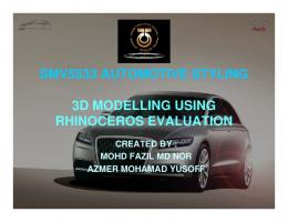
The rules for the addition;       r1 s1 r1 + s 1 r + s = r2  + s2  = r2 + s 2  , r3 s3 r3 + s 3

and scalar multiplication; r

Figure 3.1: Vector addition.

    ar1 r1 ar = a r2  = ar2  , ar3 r3

of vectors are very simple. It is easy to see that vector addition is commutative (that is the order is not important) with r + s = s + r. This is illustrated in Figure 3.1. Given two vectors r and s we define their dot product (also sometimes called their inner product) to be:     r1 s1 r · s = r2  · s2  = r 1 s1 + r 2 s2 + r 3 s3 . r3 s3

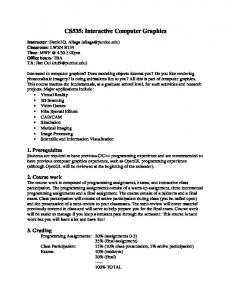
The length of a vector r, denoted krk, is given by the square root √ of the dot product of the vector with itself: r · r. The dot product can be used to generate unit length vectors using r/krk and compute the angle between two vectors: µ ¶ r·s −1 θ = cos . krkksk

u r θ

s

Figure 3.2: Vector projection.

1 There is no general convention for vector notation, Foley et al. (1993) use italicised lower case letters, while Hearn and Baker (1994) use bold upper case letters. We adhere to the more standard mathematical notation.

8


We can also project one vector, r, onto another unit vector, u. This is shown in Figure 3.2, the length of s will be given by: µ ¶ r·u ksk = krk cos(θ) = krk =r·u. krkkuk This means the dot product can be interpreted as the length of the projection of r onto u whenever u is a unit vector.

3.2

Matrices

m n

A

p * m

p =

B

Figure 3.3: Matrix multiplication.

C

n

A matrix is a rectangular array of numbers (which can be viewed as a row of vectors) which is extensively used in computer graphics since it gives us very compact notations. A general matrix will be represented by an upper case letter:   a1,1 a1,2 a1,3 A = a2,1 a2,2 a2,3  . a3,1 a3,2 a3,3

The element on the ith row and jth column is denoted by aij . Note that we start indexing at 1, whereas C indexes arrays from 0 - beware! A matrix is said to be of dimension n by m (written n × m) if it has n rows and m columns. Matrix multiplication is more complex. Given two matrices, A and B if we want to multiply B by A (that is form AB) then Pmif A is (n × m), B must be (m × p). This produces a result, C = AB, which is (n × p), with elements c ij = k=1 aik bkj , that is the i, jth element of C is the ith row of A dot producted with the jth column of B. Note that matrix multiplication is not commutative, indeed in this case we cannot multiply BA, since the sizes are wrong. /* Define the structure to hold the elements of a 3 by 3 matrices. */ typedef struct Matrix3struct { double el[3][3]} Matrix3; /* Declare the function to multiply C = AB */ Matrix3 *MatMult3(a,b,c) /* We return a pointer to a matrix. */ Matrix3 *a, *b, *c; /* These are pointers too. */ { int i,j,k; /* Do the loop to multiply the matrices - recall the zero indexing */ for (i = 0; i < 3; i++) { for (j = 0; j < 3; j++) { /* Recall we use the -> operator to access an element of a */ /* structure when we have only a pointer to that structure. */ c->el[i][j] = 0.0; /* Make sure C is initialised. */ for (k = 0; k < 3; k++) { c->el[i][j] += a->el[i][k]*b->el[k][j]; } } } return (c); } Listing 1: C code to multiply two 3 × 3 matrices.

A simple C program to perform matrix multiplication of two 3 × 3 matrices is shown in Listing 1. Matrix multiplication distributes over addition, that is A(B + C) = AB + AC, and there is an identity matrix for multiplication, denoted I, which is square and has ones on the diagonal with zeros everywhere else. The transpose of a matrix, A, which is either denoted AT or A0 is obtained by swapping the rows and columns of the matrix. Thus:   ¸ · a1,1 a2,1 a a1,2 a1,3 ⇒ A0 = a1,2 a2,2  . A = 1,1 a2,1 a2,2 a2,3 a1,3 a2,3


9

If we consider a n × 1 matrix (that is a column vector, s) then it transpose s 0 is a 1 × n matrix (which we would call a row vector). There are many other vector and matrix operators that have not been introduced here, however we shall deal with these as they are required.

3.3

2D transformations This section considers some of the transformations that are applied to 2D graphics primitives and objects. This section uses many of the results that were shown above for vectors and matrices.

Translations are simple movements or offsets from the existing position of the object. If we Before translation After translation have a point at r (a 2 by 1 column vector) and we translate it by an amount t = (t1 , t2 )0 (another Figure 3.4: 2D translation. 2 by 1 column vector) then the new location will be r ∗ = r + t. This is shown in Figure 3.4 for a rather more complex object. This is translated by applying the same translation to all the points that define the object. Scalings are simple stretchings of the object, generally about the origin. Given a point r and a scaling matrix S, where: · ¸ s 0 S= x , 0 sy where sx is the x-axis scaling and sy is the yaxis scaling the location of the new point can be written r ∗ = Sr. If sx = sy = s the scaling is said to be uniform and r ∗ = sr, otherwise the scaling is called differential. An example is shown in Figure 3.5.

Before scaling

After scaling

Figure 3.5: 2D scaling.

Rotations about the origin by an angle θ are defined by the rotation matrix R which is given by: · ¸ cos θ − sin θ R= , sin θ cos θ

Before rotation

points by θ.

3.4

After rotation

Figure 3.6: 2D rotation.

and the rotated point, r ∗ = Rr. Note that positive θ implies an anti-clockwise rotation. It is a simple exercise to show, using simple trigonometry, that R is indeed a matrix which rotates

Homogeneous coordinates

Representing 2D coordinates in terms of vectors with 2 components turns out to be rather awkward when it come to the sort of manipulation that needs to be carried out for computer graphics. Homogeneous coordinates allow us to treat all transformations in the same way, as matrix multiplications. The consequence is that our 2-vectors become extended to 3-vectors, with a resulting increase in storage and processing. Homogeneous coordinates mean that we represent a point (x, y) by the extended triple (x, y, w). In general w should be non-zero. The normalised homogeneous coordinates are given by (x/w, y/w, 1) where (x/w, y/w) are the Cartesian coordinates of the point. Note in homogeneous coordinates (x, y, w) is the same as (x/w, y/w, 1) as is (ax, ay, aw) where a can be any real number. Points with w = 0 are called points at infinity, and are not frequently used.

10


Vector triples usually represent points in 3D space, however here we are using them to represent points in 2D space, so what is going on. Well we are using a bit of mathematical trickery to make life easy for ourselves (really!). If you like then you can think of 2D space corresponding to plane w = 1. Now in homogeneous coordinates the transformations  ∗  x 1 r ∗ =  y ∗  = 0 0 1 scaling:

  sx x∗ r ∗ = y ∗  =  0 0 1 

and rotation:

  cos θ x∗ r ∗ = y ∗  =  sin θ 0 1 

can be given as: translation:   0 tx x 1 ty   y  = T r ; 0 1 1   x 0 0 y  = Sr ; 1 1

0 sy 0

− sin θ cos θ 0

  0 x 0 y  = Rr . 1 1

This is a very useful description of arbitrary translations. There are several different type of transformations. Rigid body transformations preserve length and angles (e.g. translation or rotation), while affine transformations preserve parallelism in lines (e.g. translation, rotation, scaling and shearing). A shear transformation is given by:  ∗    x 1 hx 0 x r ∗ = y ∗  = hy 1 0 y  = Hr , 1 0 0 1 1 where hx and hy represent the amount of shear along the x and y axes respectively.

3.5

Composition of transformations

One of the big advantages of homogeneous coordinates is that transformations can be very easily combined. All that is required is multiplication of the transformation matrices. This makes otherwise complex transformations very easy to compute. For instance if we wanted to rotate an object about some point, p, on (or in) that object, this can easily be achieved by: ➢ translate object by −p, ➢ rotate object by angle θ, ➢ translate object by p. This can be written as: 

1 0 T (p)R(θ)T (−p) = 0 1 0 0  cos θ =  sin θ 0

 cos θ px py   sin θ 0 1 − sin θ cos θ 0

− sin θ cos θ 0

 1 0 0  0 0 1

0 1 0

 −px −py  1

 px (1 − cos θ) + py sin θ py (1 − cos θ) − px sin θ . 1

Note that matrix multiplication proceeds from right to left. Thus to apply the composite transformation we only need apply the matrix on the right hand side to all points in the object. For those interested, Matlab provides an excellent platform for investigating these sort of transformations, since its natural matrix format makes things very easy to code.

3.6

Window to viewport transformation

In general the objects and primitives represented in the application model will be stored in world coordinates, that is their size, shape, position, etc. will be given in terms of logical units for whatever the object represent (e.g. mm, cm, m, km or light years). Thus to display the appropriate images on the screen (or other device) it is necessary to map from world coordinates to screen or device coordinates. This transformation is


11

known as the window to viewport transformation, the mapping from the world coordinate window 2 to the viewport (which is given in screen coordinates). In general the window to viewport transformation will involve a scaling and Viewport translation as in Figure 3.7 where the scalWindow ing in non-uniform (the vertical axis has been stretched). Non uniform scalings result from the world coordinate window and viewport having different aspect ratios. In Figure 3.7 the screen window (that is the viewport) covers only part of the screen. World coordinates Screen coordinates The transformation is generally achieved by a translation in world coordinates, a Figure 3.7: The window to viewport transformation. scaling to viewport coordinates and another translation in viewport coordinates, which are generally composed to give a single transformation matrix. Often the clipping of visible elements will be carried out at the same time as the transformation is applied. Typically the region will be clipped in world coordinates and then transformed. y

y

World coordinates

x

v

x

World coordinates

translation

v

Screen coordinates

scaling

u

Screen coordinates

u

translation

Figure 3.8: The procedure used to transform from world coordinate window to viewport.

The required transformations are shown in Figure 3.8. If the world coordinate window has dimensions (x min , ymin ) → (xmax , ymax ) and the viewport (or screen coordinate window) has dimensions (umin , vmin ) → (umax , vmax ), then the transformation will be given by: a translation; 

1 Tx =  0 0

0 1 0

 −xmin −ymin  ; 1

a scaling:  umax −umin

0

xmax −xmin

Sxu = 

vmax −vmin ymax −ymin

0 0

0

 0 0 ; 1

and finally another translation; 

1 Tu =  0 0

0 1 0

 umin vmin  . 1

These can be combined to yield the transformation matrix Mxu = Tu Sxu Tx =  umax −umin xmax −xmin

Mxu = 

0 0

0 vmax −vmin ymax −ymin

0

 −umin −xmin uxmax + umin max −xmin max −vmin  . −ymin yvmax −ymin + vmin 1

2 This is not the usual meaning of window as in window manager, it merely refers to the fact that we may only be taking a small window on the world, not necessarily considering infinite space.

12


3.6.1

Efficiency

The composition of transformations involving translation, scaling and rotation lead to transformation matrices M of the general form:   r1,1 r1,2 tx M = r2,1 r2,2 ty  . 0 0 1

To achieve such a transformation efficiently it should be recognised that a straight matrix multiplication of the matrix times a column vector, r = [x, y, 1]0 , is not efficient because M is sparse. This matrix multiplication would take nine multiplies and six adds. Using the fixed structure in the final row of the matrix, the actual transformation can be written: x∗ = r1,1 x + r1,2 y + tx , y ∗ = r2,2 y + r2,1 x + ty , which uses four multiplies and four adds. Since this transformation must be applied to several hundred, possibly millions, of points for each image, this can mean a big saving in computational time. However some hardware matrix multipliers (such as are present on many graphics systems) have parallel adders and multipliers which effectively removes this concern. In any case the use of homogeneous coordinates still makes sense because of the simplicity it brings to composing transformations.

3.6.2

Inverse transformations

If a general transformation (which may be composite) is given by the 3 × 3 matrix M , then the inverse transformation, which maps the new image back to the original, untransformed one is given by M −1 , that is M inverse. Since M is a matrix representing transformations this inverse matrix will exist (because a general transformation matrix is non-singular). The matrix inverse is defined so that M M −1 = I where I is the 3 × 3 identity matrix,   1 0 0 I = 0 1 0  . 0 0 1

For most transformations is is quite obvious, from first principles what the inverse transformations are, for instance the translation matrix has inverse:   1 0 −tx T −1 = 0 1 −ty  , 0 0 1

while the scaling matrix has inverse:



1 sx

S −1 =  0 0

0 1 sy

0

 0 0 . 1

If you doubt this then you can easily verify the inverse transformation matrix in Matlab. In general Matlab is a very useful tool for exploring the use 2D (and 3D as we shall see) transformations, since it was designed to be used for matrices and has extensive platform independent graphics capabilities, from drawing primitives and rendering and illumination models. If you have time I would advise you ‘play around’ with Matlab and reproduce some of the methods discussed in the notes, although this isn’t assessed.


4

13

Viewing in 3D

Most of the objects that will be stored in the application model will naturally exist in either 2D (plans, crosssections, simple graphs) or more likely 3D (real world objects, more complex graphs) space. Since the viewport is currently a 2D representation of whatever is in the application model, 3D coordinate systems call for a little extra work, defining the 2D projection of the 3D objects. First we look at defining and manipulating objects in 3D.

4.1

Geometric modelling

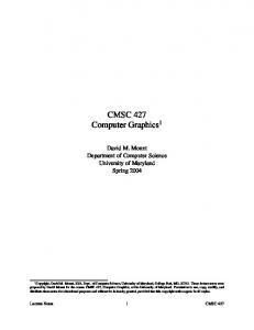
Modelling is a very familiar concept to computer scientists. We use models to represent objects, processes and abstract ideas in a way which makes understanding more simple. Graphics have a use in all modelling exercises, particularly in displaying results and conclusions. More directly, computer graphics might be concerned with different types of models such as: ➢ organisation models - hierarchies, flowcharts; directed graph representations. ➢ quantitative models - graphs, maps. ➢ geometric models - engineering and architectural structures, chemicals. In this section we confine ourselves to geometric models. As the name suggests geometric models describe the geometry of the objects which they represent. This includes: ➢ spatial layout and shape of the component parts of the object (geometry), ➢ connectivity of the component parts (topology), ➢ attributes (which affect the appearance), ➢ attributes (which pertain to the object but do not affect appearance).

robot head upper_body lower_body arm

leg feet

Figure 4.1: A hierarchical geometric robot model and its directed acyclic graph.

We commonly use hierarchical constructs to help store geometric models, because the objects we want to represent can be easily stored as a series of connected common components. The hierarchy will start with base components and combine these to form successive levels of objects. In general each object will appear in the hierarchy more than once, and the hierarchy can be symbolised using a Directed Acyclic Graph (DAG). A 2D example of a robot and its DAG can be seen in Figure 4.1. In some DAGs the arrows are omitted, since the ordering is given by the position on the page. If each object appeared only once in the hierarchy the resulting data structure would be a tree. The DAG may give details of the topology such as specifying where the objects are attached (or equivalently about which axes the objects can rotate or translate). Object hierarchies are useful because: ➢ complex models can be constructed in a simple modular fashion,

➢ stored efficiently and ➢ updated simply (the updating of one level in the hierarchy automatically updates elements below it). Figure 4.2 shows a zoomed view on the definition of the application model. We can see that the application program is composed of several subsystems which have variable degrees of access to the application model. This figure shows the logical organisation of the modules, however the actual code may be very differently organised. In many industrial application the 80/20 rule is generally true: 80% of the program deals with modelling objects (the database) and only 20% deals with producing the pictures. This view of the graphics process leads to retained mode graphics packages such as PHIGS. PHIGS is a retained mode graphics package, that is it keeps a record of all the primitives in the application model which allows automatic updating of the screen and simple editing of the primitives. Basic OpenGL, on the other hand, is

14


application code

building modification manipulation

data model

traversal for display

traversal for analysis

display and interaction handler

display device

graphics system

input device

reader and writers of the model

Figure 4.2: A closer view of the application model in the conceptual model.

an immediate mode graphics package, where only the effects on the screen are stored, not the generating primitives. PHIGS stores its information in the Central Structural Storage (CSS), a database for graphical structures. A structure in PHIGS is a sequence of elements, which are themselves primitives, appearance attributes, transformation matrices or subordinate structures. The structures define coherent geometric entities. Thus PHIGS is essentially a device independent hierarchical display list package. The CSS duplicates information in the application model, which allows fast display traversal, which is the main benefit of using a separate CSS (especially when a co-processor handles the rendering). The CSS also allows automatic pick correlation and is useful for editing the structure contained within, to produce dynamic motion (animation). This can be done by applying time varying dynamics to position, rotate or scale sub-objects within the parent objects. For instance if our parent object were a 3D robot we could use a rotation applied to a substructure (e.g. the arm) to represent joints, and dynamically rotate the arm by editing a single rotation matrix. Note that the CSS is not necessary (the application program could implement the display traversal and pick correlation - albeit at great expense) or sufficient (most real application programs will need additional data stored in the application model) for most graphical applications, it is simply an efficient way of implementing a graphics library. Thus not all graphical libraries use the retained mode principle because the overheads of duplicating the application model data and keeping the two consistent. If things change very rapidly between successive images then there will be very little benefit in using a retained mode graphics package. Thus OpenGL offers an immediate mode for such situations, and retained mode like structures (called display lists) where a CSS is more appropriate. This is covered in more detail in the lab classes.

4.2

3D coordinate systems

Much of what was discussed in the section on 2D graphics also applies here. The homogeneous coordinate system (which this time means points (or vectors) are represented by four numbers) is still very useful for manipulating transformations, but we have to take care with our coordinate system. Axis of rotation x y z

Direction of positive rotation y→z z→x x→y

Table 1: Tabular definition of the right handed coordinate system.


15

y

x

In this text we assume a right handed coordinate system, shown in Figure 4.3, where the z axis comes out of the page. This is simply a convention, and is maybe a little counter intuitive since it means that objects further away from you have a smaller z value. Beware, the z axis is taken to mean the depth (that is the depth in terms of the negative distance from the viewer) not the height as is taken is usual scientific applications. The right hand coordinate system means that a 90◦ anti-clockwise rotation about a given axis rotates one positive axis onto another:

z Figure 4.3: Right handed coordinate system.

4.3

Transformations in 3D

In 3D coordinates a general point r = [x, y, z]0 will be represented in homogeneous coordinates by r = [x/w, y, w, z/w, 1]0 , just like the 2D case. Just like the 2D case we can define transformation matrices, which will this time be 4 × 4 matrices. The transformations are: translation:    ∗  x 1 0 0 tx x ∗      0 1 0 t y y  y    r∗ =   z ∗  = 0 0 1 t z   z  = T r ; 0 0 0 1 1 1 scaling:

  sx x∗ ∗   y  0 r∗ =  z ∗  =  0 0 1 

0 sy 0 0

0 0 sz 0

  x 0 y  0    = Sr . 0  z  1 1

Rotation is a little more tricky, since we need to be careful what axis we are rotating about. A rotation about the z axis (which is basically the 2D rotation of earlier is given by:    ∗  cos θ − sin θ 0 0 x x  y  y ∗   sin θ cos θ 0 0 ∗      = Rz r , r = z ∗  =  0 0 1 0  z  1 0 0 0 1 1 a rotation about the x axis is given by:  ∗  x 1  y ∗  0 ∗   r =  z ∗  = 0 1 0

0 cos θ sin θ 0

and a rotation about the y axis is given by:  ∗  cos θ x y ∗   0 ∗   r =  z ∗  = − sin θ 0 1

0 − sin θ cos θ 0

  0 x y  0    = Rx r , 0  z  1 1

0 sin θ 1 0 0 cos θ 0 0

  0 x y  0    = Ry r . 0  z  1 1

All of the 3 × 3 upper left sub-matrices of the rotation matrices are special orthogonal which means that they preserve distances and angles. Any arbitrary sequence of rotation matrices is also special orthogonal. What is more all the above transformation matrices have inverses. For rotations, the 3 × 3 upper left sub-matrices are special orthogonal and their inverse is given by their transpose, R −1 = R0 . We can again combine the transformations  r1,1 r2,1  r3,1 0

to give a general transformation matrix M =  r1,2 r1,3 tx · ∗ ∗¸ r2,2 r2,3 ty  = R t , 0 1 r3,2 r3,3 tz  0 0 1

16


where R∗ is the 3 × 3 matrix that represents the combined effect of rotations and scalings and t ∗ is the 3 × 1 column vector representing the combined effect of all translations and 0 is a 1 × 3 row vector of zeros. Rather like in 2D efficiency can be improved by recognising that r ∗ = M r can be computed using:    x x∗  y ∗  = R ∗  y  + t∗ . z∗ z  A shear in (x, y) is given by:   1 x∗  y ∗  0 ∗   r =  z ∗  = 0 0 1 

0 1 0 0

hx hy 1 0

  x 0 y  0    = Hx,y r , 0  z  1 1

where hx and hy represent the amount of shear on the x and y axes as a function of the z value.

4.4

Transforming lines and planes

In the discussion so far we have considered the transformation of points. Lines are generally transformed by transforming the two end points separately. Planes, however, may be transformed differently. Three points define a plane and we can transform planes, much like lines, by transforming these three points. However, planes are usually defined by the (implicit) equation for a plane, f (x, y, z) = ax + by + cz + d = 0. If we define a column vector, a = [a, b, c, d]0 then writing an arbitrary point as p = [x, y, z, 1]0 points on the plane satisfy a · p = 0 or a0 p = 0. Now if we transform all points p, with a transformation matrix M , this is equivalent to transforming a so that the condition a0n p = 0 defines the transformed plane, where an = Qa and Q is the transformation matrix for a. Now: (Qa)0 (M p) = 0 , and we can now use the identity (AB)0 = B 0 A0 to write a0 Q0 M p = 0. This can only be satisfied if Q0 M = αI. Assuming α = 1 leads us to: Q = (M −1 )0 , so that the vector of coefficients, a, must be multiplied by the transpose of the inverse transformation matrix of p. Some care must be taken because there is no guarantee that M −1 will exist, particularly if the transformation represents a projection, as we will see later. In general the transformation of points, objects, planes, etc. can be most easily accomplished through combining elementary transformations using matrix multiplication. There is, however, a rather more abstract method, based on a geometrical understanding of vector operations, particularly the vector, or dot, product and the cross product. Recall that the dot product of a vector r with a unit vector u, gave the length of the projection of r onto u. Thus the projection of the vector r onto u is given by (r · u)u. The vector cross product, denoted as r × s is given by:      i s1 r1 t = r × s = r2  × s2  = det r1 s1 s3 r3

j r2 s2

 k r3  s3

 r2 s3 − r 3 s2 =(r2 s3 − r3 s2 )i + (r3 s1 − r1 s3 )j + (r1 s2 − r2 s1 )k = r3 s1 − r1 s3  , r1 s2 − r 2 s1 

where det means find the determinant of the matrix, as shown and i, j and k are unit vectors along the x, y and z axes respectively. This vector, t, is perpendicular to the plane defined by r and s and has length krkksk cos θ, where θ is the angle between r and s. Using these geometrical concepts it is possible to define the transformation matrices from first principles, although it can be rather unintuitive. For this reason we shall stick to composing elementary transformations.


4.5

17

Transformations are a change of coordinate systems

So far we have discussed transformations of objects which all lie in the same coordinate system. When this is the case we could equally as well say that the objects stayed the same, but the coordinate system was transformed - it is just another way of saying the same thing. Often this view makes more sense because the real world objects do not change position as we rotate or translate them (to reflect our motion for example), although our view of them does. However if we are stationary and the object is moving then, the former view is more logical. Consider a point p(i) in the ith coordinate system, then define the transformation between from the jth to the ith coordinate system to be Mi←j . Now: p(i) = Mi←j p(j) , and p(i) and p(j) are the same point in different coordinate systems. The coordinate system transformation matrices can be combined just like the earlier transformation matrices. One useful coordinate system transformation is given by:  1 0 0 0 1 0 MR←L =  0 0 −1 0 0 0

 0 0  = ML←R , 0 1

which transforms from a left handed to a right handed coordinate systems (and is its own inverse). The view of objects having their own coordinate systems can make a lot more sense, these being relative to some world coordinate system. In general the transformation between coordinate systems in which a point is represented will be equal to the inverse of the corresponding transformation of the set of points in a fixed coordinate system. When using multiple transformations we can use the matrix identity (AB) −1 = B −1 A−1 to work out the inverse transformation when the transformation is composite. Viewing objects as having their own frame of reference can be particularly useful when dealing with sub-objects. Considering the tricycle shown in Figure 4.4, we see that the tricycle exists in a world coordinate system, (x, y, z). The main frame the tricycle has its own coordinate system, (xt , yt , zt ) which is fixed along the tricycle but not in space. The front wheel of the tricycle also has its own coordinate system (x w , yw , zw ), which allows the wheel to rotate, and the handle bars to turn. If the tricycle moves by rotating the front wheel about the zw axis, then we need to know what do with rest of the tricycle. As the front wheel moves, both the tricycle and wheel reference frame move by a translation in x and z and a rotation about y. The tricycle coordinate system is also tied to the wheel coordinate system as the handlebars are turned. Thus to produce a full time varying model of the tricycle would be rather complex.

y y_t x z

x_t z_t

y_w

The situation is simplified if the tricycle and wheel coordinates are parallel to the world coordinate axes, and that the wheel moves straight parallel to the x axis. As z_w the front wheel rotates by an angle θ, a point, p, on the wheel moves by an amount θr, where r is the radius of the wheel, and thus the tricycle moves forward θr Figure 4.4: A simple tricycle. units. Thus the point on the wheel has rotated about the wheel z axis by an angle θ and moved forward a distance θr. The coordinates of the new point in the original wheel coordinate system are: x_w

p∗(w) = T (θr, 0, 0)Rz (θ)p(w) , while the coordinates in the new, translated, wheel coordinate system are: 0

p∗(w ) = Rz (θ)p(w) . To find the point in world coordinates we need to transform from wheel coordinates to world coordinates. Thus: p∗ = M·←w p(w) = M·←t Mt←w p(w) ,

18


that is we can convert to the world coordinate system by going from wheel to tricycle and then tricycle to world coordinate systems. Both these transformations are given by translations given by the initial position of the tricycle. Thus the new point in the world coordinate system is given by: p∗ = M·←w T (θr, 0, 0)Rz (θ)p(w) . There are other ways to represent this. In general if we were to represent the tricycle we would use the equations of motion of the tricycle to update M·←w0 and Mt0 ←w0 and then use these to determine the world coordinates of the updated points on the tricycle expressed in local coordinates.

4.6

Projection

This is possibly the most difficult section of these notes. However since many of the objects which exist in the application model will naturally be represented in a 3D coordinate system, and the screen is 2D, projection is a necessary part of any graphics module. 3D world coordinate output primitives

Clip against view volume

Project onto projection plane

Transform to 2D device coordinates

2D device coordinates

Figure 4.5: The procedure used to transform from 3D world coordinate window to the 2D viewport.

In Figure 4.5 we see that projection is only one part of the chain necessary for displaying a 3D application model on a 2D screen. The first step involves clipping against a 3D view volume, to remove those objects that are behind us or too distant to be visible. We then need to define the projection we wish to use and the viewing parameters, and apply this to the clipped part of the application model. Finally we transform to screen coordinates, in the manner we have already addressed.

to

Projections are general mappings that transform a nD coordinate syspro pro tem into a mD coordinate system. ject ject ion C A ion plan plan Almost all useful projections involve e e m < n, and in computer graphC* ics n = 3 and m = 2 most if the A* D B time3 . The projection of a 3D object is described by straight ‘proors rs B* t jection rays’ (called projectors), c o t je D* ec pro oj which emanate from the centre of pr the projection, pass through all centre of projection points in the object and intersect the projection plane to produce the ‘image’. The centre of projection is generally at a finite distance Figure 4.6: A perspective projection (left) and a parallel projection (right). from the projection plane (giving perspective projections), but is sometimes defined at infinity (giving parallel projections – see Figure 4.6). ty

ini

inf

We consider planar geometric projections since the surface we are projecting the objects onto is a flat plane. Perspective projections require the definition of the centre of projection, which will be a point, p, with homogeneous coordinates [x, y, z, 1]0 . A parallel projection is defined by a direction (which can be expressed as the difference of two vectors; [x, y, z, 1]0 −[x∗ , y ∗ , z ∗ , 1]0 = [a, b, c, 0]. Recall that points expressed in homogeneous coordinates with w = 0 are called points at infinity, and also correspond to directions. When we, as humans, view the world we experience something known as perspective foreshortening, which is very similar to the effect produce by a perspective projection. Perspective foreshortening means that the size of the project object varies as one over the distance to the object. What is more perspective projections are not very useful for representing exact shapes, since angles for all objects other than those parallel to the plane of projection are distorted, distances cannot be measured from the projection, and parallel lines are not preserved. The view is, 3 In scientific visualisation it is not uncommon for n to be equal to 100, for instance, but we shall not consider these problems here.


19

however, more visually realistic. Parallel projections also distort angles, but maintain parallelism and distances. Parallel projections look less realistic.

4.6.1

Perspective projections In a perspective projection all parallel lines that are not parallel to the projection plane appear to go to a vanishing point, which will only be reached at infinity. If the set of parallel lines is also parallel to one of the principal axes, the point at which the lines meet is called an axis vanishing point. The number of axis vanishing points will depend on the number of axes cut by the projection plane. The number of axis vanishing points defines the type of the perspective projection. Figure 4.7 shows the one (vanishing axis) point projection of a cube onto a plane that only cuts the z axis.

y Projection plane

x Center of projection z

Figure 4.8 shows a two (vanishing axis) point projection of the cube, where the projection plane cuts x and z axis but is parallel to the y axis. Note the two vanishing points for the x and z axes as well as the centre of the project, which in this case (and generally) will be different. Three point projections are used rather less regularly, since two point projections are generally sufficiently realistic.

Projection plane normal

Figure 4.7: One point perspective projection of a cube (from Foley et al. (1993)).

y

Projection plane

z x

x-axis vanishing point

z-axis vanishing point

Center of projection

Figure 4.8: A two point perspective projection of a cube (from Foley et al. (1993)).

20


4.6.2

Parallel projections Projection plane

Projection plane

y

y Projector

Projector

z

Projectionplane normal

x

x z (a)

Projection-plane normal

(b)

Figure 4.9: (a) A isometric projection of a cube, (b) an oblique projection of a cube (both from Foley et al. (1993)).

Projection plane (top view) Projectors for side view Projectors for top view

Projectors for front view

Projection plane (side view)

Projection plane (front view)

Figure 4.10: Three orthographic projections of a ‘house ’ (from Foley et al. (1993)).

Parallel projections can be divided into two categories: orthographic and oblique. Parallel orthographic projections have the direction of the projection parallel to the normal to the projection plane, as shown in Figure 4.10. These projections are frequently found in architecture and engineering drawings where three views are recognised: front elevation, plan elevation and side elevation. In these cases the projection plane is parallel to a principal axis. Axonometric orthographic projections are parallel projections that use projection planes that are not normal to the principal axes. This projection preserves parallel lines but not angles and distances. An isometric projection is a frequently used axonometric orthographic projection in which the projection plane normal makes equal angles with the principal axes. There are only eight possible directions for isometric projects,

an example being shown in Figure 4.9(a). A different form of parallel projection is the so called oblique projection. In these the projection plane normal and direction of projection differ. The projection plane is still normal to the principal axes, and thus for objects parallel to the projection plane distances and angles are preserved. They are frequently used to illustrate 3D objects in texts (e.g. largely used in Foley et al. (1993)). There are many types of oblique projection but we do not consider them here.

4.6.3

Specification of 3D views

Recall that Figure 4.5 showed two stages to the 3D to 2D transformation, first a clipping, then a projection. The clipping is achieved by defining a view volume (the volume that can be seen). This section considers the specification of a view volume. The projection plane (which is called the view plane in the graphics literature - a term we shall henceforth adopt), is defined by the View Reference Point (VRP), a point on the view plane, and the View Plane Normal (VPN), a normal to the view plane. Note that the view plane can be anywhere with respect to the objects in the application model - behind, in front of or even cutting through. Given we have the view plane (which defines an infinite 2D region) we now need to define a view window, so that objects outside the window are not displayed. Defining a view window requires us to define two principal axes in the view plane and then the maximum and minimum coordinates of the view window. The axes are an integral part of the Viewing Reference


21

v View plane VUP

VRP VPN u

n

Figure 4.11: Definition of the view plane (from Foley et al. (1993)).

Coordinate (VRC) system. The VRC has the VRP as it’s origin, with the n axis defined by the VPN. The v axis of the VRC is defined by the View Up Vector (VUP), and thus the u axis follows from the assumption of a right handed coordinate system, as shown in Figure 4.11. The VRP (point) and VPN and VUP (directions) are specified in a right handed world (application model) coordinate system. The view window is then defined by (umin , vmin ), (umax , vmax ).

View plane

v

View plane

DOP

CW

VRP

CW

VPN u

n

VRP PRP

Center of projection (PRP)

VPN n

(a)

(b)

Figure 4.12: Definition of the infinite view volume from Foley et al. (1993): (a) perspective projection, (b) parallel projection.

The centre of projection and Direction Of Projection (DOP) are defined by a Projection Reference Point (PRP) and an indicator of the projection type (see Figure 4.12(a)). If the projection is a perspective projection the the PRP is is the centre of projection. If the projection is parallel, the the DOP is defined by the direction between the PRP and the centre of the projection window (CW in Figure 4.12(a)). The coordinates of the PRP are defined in the VRC, not world coordinates, which means the PRP does not change (relative to the VRP) as the VUP and VRP are changed. This means that it is simpler for the programmer to change the direction of projection required, at the expense of extra complexity if the PRP is moved (i.e. to get different views of the object). The view volume of a perspective projection is the infinite volume defined by the combination of the PRP and the view window (Figure 4.12(a)), which defines a pyramid. This can be contrasted to the view volume for a parallel projection which gives an infinite parallelepiped ((Figure 4.12(b)). In general we will not want the view volume to be infinite, rather we will want to limit the number of output primitives which are displayed. Figure 4.13 shows how finite volumes are defined by selecting the signed quantities F and B which define the locations of the front and back clipping planes (also called the hither and yon planes). Both these planes are parallel to the view plane, thus F and B are defined along the VPN. By changing the distances F and B it is possible to give a good feeling for the 3D shape of an object, almost as if we could slice through it. To display the contents of the view volume the objects mapped into a unit cube whose axes are aligned with the VRC system (called the normalised projection coordinates), giving us the 3D viewport, which is contained within a unit cube. The z = 1 face of this unit cube is then mapped to the largest square that can be displayed (in display coordinates). To create a wire-frame display of the contents of the 3D viewport we can simply drop

22


Back clipping plane Front clipping plane

View plane

Front clipping plane

View plane

Back clipping plane

VRP

VRP VPN DOP

VPN

B

F

B (a)

F

(b)

Figure 4.13: Definition of the finite view volume (from Foley et al. (1993)).(a) perspective projection, (b) parallel projection.

the z coordinate. For more complex displaying methods, such as applying hidden line removal algorithms we must retain the z coordinate. In general two matrices are used to represent the complete view specifications; the view orientation matrix and the view mapping or view projection matrix. The view orientation matrix gives information about the position of the viewer relative to the object and combines the VRP, VPN and VUP. The 4 × 4 matrix then transforms positions represented in world coordinates to positions represented in the VRC, that is we map the u, v, n axes into the x, y, z axes respectively (note the coordinate change is reversed). The view mapping matrix uses the PRP, view window and the front and back distances to transform points in the VRC to points in normalised projection coordinates, as we shall see next.

4.7

Implementing 3D→2D projections

This section contains the details necessary to implement (and understand) understand planar geometric projections. Rather than get involve with a mathematical derivation this section gives details of the mathematics required to implement the methods. By working back from this, those students that wish to can gain a better understanding of the mathematics as well. The overall aim here is to define normalising transformations Npar (parallel) and Nper (perspective) that transform the points in world coordinates within the view volume to points in the normalised projection coordinates. From these we can apply clipping algorithms and 3D to 2D projections in a simple manner. This essentially adds a preprocessing step to Figure 4.5. We treat the parallel and perspective cases separately, although as you will see there are a lot of similarities.

4.7.1

Parallel projections

In this case our canonical view volume (created by the mapping into normalised projection coordinates) is the unit parallelepiped defined by the planes, x = −1, x = 1, y = −1, y = 1, z = 0 and z = −1. Here we derive the transformation matrix Npar for very general parallel projections, which may be oblique. The steps necessary to achieve a canonical view volume are: 1. Translate the VRP to the origin. 2. Rotate the VRC such that it is aligned with the world coordinate system. 3. Shear (in x and y) so that the direction of projection is aligned with the z axis. 4. Translate and scale into the canonical view volume (parallelepiped).


23

To implement these transformations all at one go would require a lot of mathematical analysis, however using homogeneous coordinates we can easily create the necessary individual steps 1 to 4 and combine the transformation matrices. Steps 1 and 2 combined produce the view orientation matrix, while steps 3 and 4 give the view mapping matrix. Step 1: Translate the VRP (that is the point at which world coordinates, so the translation is simply:  1 0 T (−V RP ) =  0 0

we are ‘looking’) to the origin. The VRP is specified in 0 1 0 0

 −vrpx −vrpy   . −vrpz  1

0 0 1 0

Step 2: Rotate the VRC such that it is aligned with the world coordinate system. The row vectors of the rotation matrix to perform this transformation are the unit vectors that are rotated by R into the x, y and z axes. The VPN is rotated into the z axis, so Rz =

VPN . kVPNk

Similarly (recalling that the vector cross product gives vectors that are orthogonal to both input vectors) we can rotate u to x giving VUP × Rz Rx = . kVUP × Rz k Finally the v axis is rotated into the y axis:

Ry = R z × R x , where the result is already normalised since both Rx  r1,x r1,y  R= r1,z 0

and Rz are. The final rotation matrix is given by:  r2,x r3,x 0 r2,y r3,y 0  . r2,z r3,z 0 0 0 1

The derivation is rather tricky, but the concept of rotating the two coordinate systems (world and view reference) so that they are equivalent is logical. y

y

DOP shear

DOP’

VPN -z

-z

VPN

Figure 4.14: Shearing the view volume so that the direction of projection (DOP) is parallel to the z axis (side view).

Step 3: Shear (in x and y) so that the direction of projection is aligned with the z axis. The details of the derivation of the correct shear parameters can be found in Foley et al. (1993, p. 219). The direction of projection is the vector from the PRP to the centre of the view window. Thus the vector can be written:   umax −umin   dopx − prpu 2 dopy   vmax −vmin − prpv  2    , DOP =  dopz  =   −prpn 0 0 noting that previous transformations mean that the matrix required is given by:  1 0 Hpar =  0 0

world coordinates and VRC are the same thing. The shear x 0 − dop dopz dopy 1 − dopz 0 1 0 0

 0 0  , 0 1

24


Step 4: The transformation to canonical coordinates. This step is not necessary for display, however most clipping algorithms require a canonical volume element, and it makes projection easier. Essentially we need to centre the view volume at the origin and then scale so that it has the correct dimensions. The matrix to achieve the translation is:   min 1 0 0 − umax +u 2 0 1 0 − vmax +vmin  2  , Tpar =  0 0 1  −F 0 0 0 1

and the scaling is:



2 umax +umin

 Spar =  

0 2 vmax +vmin

0 0 0

0 0

0 0 1 F −B

0

 0 0  . 0 1

We can now write the matrix for performing arbitrary parallel projections as Npar = Spar Tpar Hpar RT (−V RP ), that is the composition of several simple individual transformations.

4.7.2

Perspective projections

For perspective transformations a slightly different combination of transformations is needed to obtain a canonical view volume. These are: 1. Translate the VRP to the origin. 2. Rotate the VRC such that it is aligned with the world coordinate system. 3. Translate so that the centre of projection (i.e. the PRP) is at the origin. 4. Shear (in x and y) so that the direction of projection is aligned with the z axis. 5. Scale into the canonical view volume (truncated pyramid). Steps 1 and 2: same as those in the parallel case. Step 3: the translation of the centre of projection (i.e. the PRP) to the origin. This step is given by: 

1 0 T (−P RP ) =  0 0

0 1 0 0

 −prpu −prpv   . −prpn  1

0 0 1 0

Step 4: same as step 3 in the parallel case. Step 5: Scale into the canonical view volume (truncated pyramid). The scaling matrix is given by: 

  Sper =  

−2prpn (umax −umin )(B−prpn )

0 0 0

0 −2prpn (vmax −vmin )(B−prpn )

0 0

0 0 1 prpn −B

0

 0  0  . 0 1

The reasoning behind the structure of Sper can be found in Foley et al. (1993, p. 225–226). The final composite transformation matrix is given by Nper = Sper Hpar T (−P RP )RT (−V RP ). Note that both Npar and Nper will not affect the homogeneous coordinate w since they are combinations of translations, rotations, scalings and shearings, so division by w is not normally necessary to return to 3D coordinates.


25

It is often useful to add an additional step to the computation of Nper transforming the truncated pyramid to a parallelepiped so that the same clipping algorithms can be used for parallel and perspective projections. This transformation matrix is given by:   1 0 0 0 0 1 0 0   M = −zmin  , 1 0 0 1+zmin 1+zmin 0 0 −1 0 where zmin = (prpn − F )/(B − prpn ). Using M we can create a new perspective transformation matrix which ∗ = M Nper . maps the objects into the rectangular canonical view volume: Nper

4.7.3

Clipping

Once the application model has been projected into a canonical view volume the clipping of objects can be undertaken in two ways, either in 3D coordinates or homogeneous coordinates. We do not have time to deal fully with this subject, details can be found in Foley et al. (1993).

4.7.4

Projection

After the objects have been clipped we can project the remaining elements from the 3D canonical volume into 2D coordinates. This is achieved by using an appropriate transformation matrix. For the parallel projection case, the orthographic projection matrix is:   1 0 0 0 0 1 0 0   Mort =  0 0 0 0  . 0 0 0 1

For a perspective projection the transformation matrix  1 0  Mper =  0 0

is given by:  0 0 0 1 0 0  , 0 0 0 0 d1 1

where d = −1 having performed the transformation using Nper .

4.7.5

Viewport transformation

The objects transformed following matrices:  1 0 0 0 1 0  0 0 0 0 0 0

by the projection will then be transformed into the viewport coordinates using the   xvmax −xvmin xvmin 2  yvmin  0  zvmin   0 1 0

0 yvmax −yvmin 2

0 0

0 0 zvmax −zvmin 1

0

 0 1  0  0 0  0 0 1

0 1 0 0

0 0 1 0

 1 1  . 1 1

This moves the origin of the canonical view volume to (0, 0, 0), scales by the viewport dimension and then translates to the viewport origin. To plot the resulting 2D object we divide by w and then simply ignore the z coordinate and plot the x and y coordinates.

26


4.7.6

Overview

There was a lot of material in this section. To summarise the process of 2D viewing of 3D objects is given by: ➢ 3D → homogeneous, ➢ apply Npar or Nper , ➢ homogeneous → 3D, ➢ clip, ➢ 3D → homogeneous, ➢ project using Mort or Mper , ➢ transform into device coordinates, ➢ homogeneous → 2D.

It is not always necessary to apply all these steps, for instance in some case clipping may not be very important (for instance when the application model only contains a small amount of information), and the steps related to clipping may be omitted. The series of projections outlined in this section are those which are used across all systems, however you should be aware that different terms are used for some of the coordinate systems, in different graphics libraries.


5

27

Surface Modelling

So far in this course, simple wire-frame graphics have been the focus. In this section we extend the wire-frame model to allow for surfaces and thus the illusion of solid objects. In this section we consider only surfaces composed of planar objects, in the next section we briefly develop methods for curved surfaces. The area is related to the concept of solid modelling, which involves the representation of volumes. Surface models are often used to specify the bounding elements of the solid object.

5.1

Polygonal Meshes

A polygonal mesh is a set of connected planar polygons (often triangles) which are used to represent the surface of an object. Because we are restricted to planar geometry these work best on naturally planar (typically man made) objects. However by specifying a sufficiently large number of very small polygons it is possible to approximate curved objects to arbitrary accuracy, at the expense of greatly increased data and processing cost. Within a polygonal mesh each polygon edge is shared by only two polygons. An edge always connects two vertices, and the polygon is a closed sequence of edges (that is the start and end vertices are the same). Also every edge must be part of some polygon. There are several possible representations for a polygonal mesh, the most appropriate one being determined by the specific part of the application for which it is to be used. Often several representations will be used within the same program, one for external storage, one for internal use and possibly one for interactive mesh definition. As with most software problems there will be a space-time tradeoff for each representation. In general the more information on the structure of the mesh (that is the relations between the edges, vertices and polygons) the greater the space requirements, but the faster the processing of queries such as finding all the edges of a given polygon, finding both polygons of a given edge, or finding the vertices connected to a given edge. The explicit representation defines each polygon P as: P = {(x1 , y1 , z1 ), . . . , (xn , yn , zn )} , where the vertices are stored in the order in which they would be encountered were we to move around the edge of the polygon. This is fine (space wise) for one polygon, however if we have more than one polygon they will have at least one shared edge, so there is unnecessary duplication. What is more there is no topological information here, that is there is no explicit information on shared edges or vertices. Also if we wanted to display the mesh as filled or outline polygons we would need to transform and clip each vertex and edge of each polygon. Then when the mesh was displayed each edge would be drawn twice. An alternative method, known as the pointers to a vertex list method uses a technique whereby each vertex in the polygon mesh is stored just once. This creates a vertex list:

V1 E1

E5 V4

P2

E3

P1

E4

V2 E2

V3 Figure 5.1: A polygon mesh.

V = {(x1 , y1 , z1 ), . . . , (xn , yn , zn )} , where n might be very large (this contains the vertices for all polygons). Each polygon is then represented as a series of pointers to vertices in the vertex list, P = {V1∗ , . . . , Vn∗ }. While this structure has reduced the storage requirements, it is still not very efficient for finding polygons that share edges and the edges will be drawn twice if all polygons are drawn.

The solution is to use a pointers to an edge list, which keeps the vertex list V , but adds an edge list E which stores all the edges using pointers to the two end vertices and to the polygons which the edge is part of. We also store the polygons as pointers to members of the edge list. An example is shown in Figure 5.1 where the vertex list V = {V1 , V2 , V3 , V4 } = {(x1 , y1 , z1 ), . . . , (x4 , y4 , z4 )} and the edge list is E1 = {V1∗ , V2∗ , P1 , O}, E2 = {V2∗ , V3∗ , P1 , O}, E3 = {V3∗ , V1∗ , P1 , P2 }, E4 = {V3∗ , V4∗ , P2 , O} and E5 = {V4∗ , V1∗ , P2 , O} where O represents the null or external polygon. Finally the polygon list would be P1 = {E1∗ , E2∗ , E3∗ } and P2 = {E3∗ , E4∗ , E5∗ }. We have

28


used ∗ to denote the fact we store a pointer to the objects, rather than the objects themselves. When displaying the polygon mesh the edges are drawn, which means there is no repetition of edges. The transformations will be applied to the vertex list, while clipping and scan conversion can be done using the edges. However it is still difficult to determine which edges are connected to a given vertex - all edge lists must still be examined - unless we add extra information explicitly.

5.2

Solid modelling

This section gives a very brief introduction to the concepts and methods used in modelling solid objects. This is important in CAD/CAM applications and the generation of photo-realistic images. The details of the implementations will not given but the interested reader can refer to Foley et al. (1993) or Hearn and Baker (1994). Further detail can be found in Foley et al. (1996). The essential difference between solid modelling and surface modelling is that we have to know the difference between the inside and the outside of a solid model. So what capabilities should a solid model have? It should cover a domain of representation that is large enough to embody those objects which we might reasonably want to model. The representation should be unambiguous or complete in that given a particular representation there is only one solid that corresponds to it. We would also like it to be unique so that a given solid can only be represented one way. It might also be desirable that the representation is accurate so that the model is an exact representation of the object. Some types of model only allow straight lines, others can be used with curved surfaces. If the representation can ensure it is impossible to create an invalid object it will save us time having to check for validity. It should allow easy construction of the model. The representation should be closed under under rotation, translation and other operations, so that a transformed solid is still a solid. The representation should also be compact and efficient. It should be clear from this long list of requirements that no single system will satisfy all requirements simultaneously, thus there are trade-offs with every representation.

B

A (a)

(b)

(d)

(c)

(e)

Figure 5.2: Boolean operation on solids. (a) Objects A and B, (b) A ∪ B, (c) A ∩ B, (d) A − B, (e) B − A (from Foley et al. (1993)).

Just like the 2D case, we can define the standard Boolean set operators for 3D solids, as shown in Figure 5.2. Some care has to be taken since the application of a Boolean operator to two solids may not produce a solid. The regularised Boolean operators are defined in such a way as to ensure that their application always yields solids. For example the regularisation of the intersection of two cubes which only meet at a vertex is the null object.

(a)

(b)

(c)

(d)

Figure 5.3: The regularisation of an object. (a) The original object, (b) the closure of the object, (c) the interior of the object and (d) the regularisation of (a). (from Foley et al. (1993)).

The concept of regularisation can be seen in Figure 5.3. The boundary points of an object are those which have zero distance from the object and it’s complement. A closed set contains the boundary points, while an open set does not. The union of the set and it’s boundary is called the closure. The regularisation of a set is the closure of the set’s interior points. We will now briefly review some of the more common solid representations.


5.2.1

29

Primitive instancing

As the name suggests, when using primitive instancing a set of primitives is defined by the model, which are directly relevant to the objects which the application should represent. For instance if the object is an engine, then the primitives might consist of pistons, rods, chains and cogs. This implies a rather high level specification, the primitives themselves may be rather complex to define.

5.2.2

Sweep representations

Sweep representations use a 2D planar template (cross-section) to define the profile of the object. This is then swept along a path, normal to the plane of the 2D template, to generate the 3D element. In translational sweeps or extrusion the sweep path is a straight line, and a 3D extension of the 2D template is produced. This can be modified by applying transformations to the 2D template as the template moves along the line that defines the translational sweep. Often the sweep path is circular, generating a rotational sweep, which can be used to produce objects with some form of rotational symmetry about at least one of their axes. The method can be generalised to sweep 3D objects. Note that the set of solids produced by even simple translational sweeps is not close under the Boolean set operation of union, since the union of 2 sweeps is in general not a sweep itself (because the symmetry will be broken unless the lines of sweep of both objects are parallel).

5.2.3

Boundary representations Boundary representations or b-reps describe the solid object in terms of its boundaries, that is the vertices, edges and faces. We will only consider planar b-reps, however curved surfaces can be represented within the same framework, although it is common to represent curved surfaces as a series of planar faces (c.f. finite elements). This uses representation methods that are very similar to those discussed in the Section 5.1.

Most b-rep systems can only represent shapes that have boundaries that are 2-manifolds. This means that an edge can be shared by at most 2 faces. A polyhedron (which beFigure 5.4: Simple polyhedra. longs to the set of objects having 2-manifolds) is a solid which is bounded by a set of polygons whose edges belong to only one other polygon. A simple polyhedron has no holes in it - that is it can be transformed into a sphere without breaking any of the connectivity. Euler’s formula tells us that for a simple polyhedron with V vertices, E edges and F faces, V − E + F = 2 (see Figure 5.4). This gives us necessary conditions for an object to be a simple polygon, but not sufficient conditions since there exist objects for which Euler’s formula is satisfied, but which are not simple polyhedra. Sufficient conditions are given by ensuring that each edge only connects two vertices and is shared by only two faces, faces do not inter-penetrate and at least three faces meet at each vertex. V=8, E=12, F=6

V=5, E=8, F=5

One advantage of the b-rep system is that b-reps can be combined using the regularised Boolean set operators, such as union, to produce new b-reps, although this can be rather complicated to implement.

5.2.4

Spatial partitioning representations

Spatial partitioning representations divide the solid to be represented into a number of primitive solid objects, which are more simple than the object. One of the most general forms, known as cell decomposition represents the object as a number of small, simple cells - which will often be parametrically represented and curved. Combining these cells in a bottom-up fashion allows us to define more complex objects. Combining the cells, sometimes called gluing, is like a union, but must ensure that the objects do not intersect.

30


Spatial occupancy enumeration is a special case of cell decomposition where only one type of cell (typically a cube) is used on a fixed, regular grid. The cells, often referred to as voxels (volume elements), represent a discrete version of the object and have the problems that we met earlier in the transformation from 2D objects to pixels. There is also the problem of storage space since the amount of information need grows as n 3 if n is the number of voxels along each axis. The storage requirements can be reduced by using octrees which applies a binary subdivision in a divide-and-conquer algorithm. In general the number of nodes in an octree (which gives the amount of storage needed) will be proportional to the objects surface area, which is of order n 2 rather than n3 . There has been a lot of work done on the processing (by Boolean set operations) of octrees and efficient algorithms exist. To visualise the implementation of an octree, it is easier to understand it’s 2D equivalent, the quadtree (Figure 5.5). In a quadtree the cells are squares, with each square being divided into four smaller squares at each level of the tree. Figure 5.5 shows the use of a 3 level quadtree to represent a planar object shown by the thick black line. A node in the quadtree can either be partially covered by the object (P), fully covered (F) or not covered (E). By defining the first leaf to be the lower left hand square of the division of the node above, the full information can be stored by just 3 values at each node. The leaf nodes will always be F or E. Since the position of the nodes is fixed, there are some problems with using these sort of models (which are also used widely in image processing where they are referred to as tree based models.)

P P

F

P

E

Binary Space-Partition (BSP) trees divide space into two using arbitrary planes. BSP trees were originally developed to aid visible surface E F E E E E E F determination. Each internal node of the BSP tree is associated with a plane and has two children, inside and outside (for each side of the plane). Figure 5.5: A simple quadtree. If the normal points out of the object then the left child is behind the plane (inside) and the right child is in front of the plane (outside). The construction of BSP trees is rather complex and we do not address it further here. More information can be found in Foley et al. (1993, p. 386).

5.2.5

Constructive solid geometry

In constructive solid geometry the solid is defined using the regularised Boolean operations on some simple primitives such as shown in Figure 5.6. The means by which the primitives in the representation are specified varies across implementations. It is clear that cell decomposition and spatial occupancy enumeration can be viewed as special cases of the constructive solid geometry model.

U*

–*

5.2.6

–*

Which model to use?

Clearly there are several models which one could use to model a given solid. Which model is best will depend Figure 5.6: The use of constructive solid geomeupon many considerations, as outlined at the start of try. (from Foley et al. (1993)). this section. For instance spatial partitioning and b-rep (with polygonal planar boundaries) will not be very accurate for curved objects (although if we take smaller and smaller divisions we can minimise this at the cost of increased storage and computation). Foley et al. (1993, p. 390) gives a more complete discussion of the merits of the various approaches. Another issue in solid modelling is that of the definition of the solids in the first place. This can be done mentally for simple objects, however for more complex tasks, such as the display of a room, automated or computer assisted methods will be necessary.


6

31

Curves

So far in the course we have dealt only with models which use straight lines or planar surfaces. Natural objects have a variety of possible shapes, some curved and some very irregular (but often repetitive at the fine scale fractals). In the first part of this section we deal with curves in 2D. The second part outlines the specification of smooth surfaces in 3D.

6.1

2D curves

Most of the curves used in computer graphics are parametric curves, that is the position of the curve in (x, y) space is given by some parameterised function. The explicit form of the functions, such as y = f (x), are generally not appropriate because: ➢ it is impossible to get multiple y values for a given x value, ➢ the form is not rotationally invariant and, ➢ you cannot describe curves with a vertical tangent. The implicit form of a function, such as f (x, y) = 0, is not very suitable for representing curves either because: ➢ the given equation may have more solutions than we want, ➢ to restrict the solution to one branch we need extra constraints, ➢ joining curves can be a problem. Thus a third form of curve, know as a parameterised function is used to represent general 2D curves. Here we let x = x(t) and y = y(t) where t is some index which you can think of as time or distance along the curve. The most commonly used type of parametric curve is the piecewise cubic polynomial curve. This is much like the polylines (piecewise continuous linear objects) used in earlier sections, except the individual elements are now cubic functions of t. Cubic polynomials are often used because they are sufficiently flexible to approximate general curves but do not have too many coefficients (parameters).

6.1.1

Piecewise cubic polynomial curves

3

The general form of a curve segment is given by q(t) = (x(t), y(t))0 where:

2 1

x(t)

=

a x t3 + b x t2 + c x t + d x ,

0

y(t)

=

a y t3 + b y t2 + c y t + d y .

−1 −2 −3 −4 −5 −4

−2

0

2

Figure 6.1: A sample of cubic pieces.

4

We restrict t ∈ [0, 1]. Some examples are shown in Figure 6.1. Using matrix and vector notation we can write:  3 3 t t · ¸  t2 t2  a x bx c x d x   t= , C= , t t a y by c y d y 1 1

so that q(t) = Ct, giving a compact notation. It is clear that this representation can be used for a single curve segment, but how do we join curve segments? Well ideally we would like the curve segments to join (that is we would like continuity) and we would like the curves to have the same slope when they join (smoothness, also called continuity of the derivative). We ensure continuity and smoothness by matching the derivatives (or slopes) of the curves at the joining points. Thus we compute: ¶ µ ∂(Ct) ∂x(t) ∂y(t) ∂t ∂q(t) = = , =C , ∂t ∂t ∂t ∂t ∂t

32


where: 3t2 ∂t  2t = ∂t  1 0 

 3t2 2t   . 1  0

It is possible to define many types of continuity: ➢ G0 geometric continuity - the curves join ➢ G1 geometric continuity - the curves join with equal tangent directions. ➢ C 1 continuity - the curves join with equal tangent directions and magnitude (first derivatives equal). ➢ C n continuity - the curves join with equal n’th derivatives. If we consider t to be time, then C 1 continuity implies that the velocity of an object moving along the curve is continuous. It will often also be useful to enforce C 2 continuity on the curve so that the acceleration is also continuous. For instance if the curve were to represent the path of an artificial camera it might look rather odd if the acceleration suddenly changed across the piecewise segments. So how do we join the segments? There are four unknowns for each of x and y thus we require four constraints to determine the system of equations at each segment. The constraints we have are: ➢ constraints on end points, ➢ constraints on tangent vectors (derivatives), ➢ and constraints on continuity between segment end points. In this section we will consider three main types of curve: ➢ Hermite – defined by two end points and the tangent vectors at the end points, ➢ B´ ezier – defined by two end points and two control points which determine the tangent vectors at the end points, ➢ B-splines – defined by four control points, with C 2 continuity. 6.1.2

Hermite curves 1.2

A Hermite polynomial form is specified by the definition of two end points p1 , p4 and two end tangent vectors, r 1 , r 4 . The question is how do we determine the coefficients of the polynomials, that is the matrix C given these constraints? The answer is complex but when followed in a step by step fashion it should be comprehensible.

1

BH(t)

0.8 0.6 0.4 0.2

The essential step is that we expand C into two matrices. Let us consider the row of C that corresponds to the x coefficients, Cx . We can write:

0 −0.2 0

0.2

0.4

0.6

0.8

1

t

x(t) = ax t3 + bx t2 + cx t + dx = Cx t = Gx MH t ,

Figure 6.2: The Hermite basis functions.

where Gx is the x-component of the so called geometry matrix, which is given by the constraints and M H is the Hermite basis matrix which defines the basis functions used to represent the function x(t). We know what Gx is - it is simply [p1,x p4,x r1,x r4,x ] from the constraints (this is the definition of G). Thus we can determine MH using the above equations as outlined in Foley et al. (1993, p. 333). This yields:

MH



2 −2  = 1 1

−3 0 3 0 −2 1 −1 0

 1 0  . 0 0

We can now write x(t) in two ways; either as a function ax t3 + bx t2 + cx t + dx or as a linear combination on finite support non-linear basis functions Gx BH (t) where BH (t) = MH t are the Hermite blending functions. The basis (or blending) functions for Hermite polynomials are shown in Figure 6.2. Note this is the only time you might see the curves plotted as a function of t, since in real applications x is plotted against y.


33

Now given the geometry matrix, G, and given that we know the Hermite basis matrix, M H , we can compute C = GMH . To draw the curves we simply evaluate x(t) and y(t) at successive values of t, where the step size is kept small. Hermite curves are often used in graphics packages for specifying smooth curves.

6.1.3

B´ ezier curves 1

0.8

0.6 B

B (t)

Bézier curves are very similar to Hermite curves except that we use four control points, p1 , p2 , p3 and p4 . The intermediate control points give the starting and ending tangent vectors, so that r 1 = 3(p2 − p1 ) and r 4 = 3(p4 − p3 ). Thus the Bézier geometry matrix is Gx is - it is simply [p1,x , p2,x , p3,x , p4,x ]. This means that the B´ ezier basis matrix will be:   −1 3 −3 1  3 6 3 0  MB =  −3 3 0 0 . 1 0 0 0

0.4

0.2

0 0

0.2

0.4

0.6

0.8

1

t

Figure 6.3: The Bézier basis functions.

Again we can compute the basis (or blending) functions which are shown in Figure 6.3. These basis functions are known as Bernstein polynomials. Note that the Bézier curve is completely contained within the convex hull defined by the four control points. If we need to join two Bézier curves, with control points p1 , p2 , p3 , p4 (in both), p5 , p6 , p7 , then we will need an extra condition to ensure G1 or C 1 continuity. Having p4 in both curves ensures G0 or C 0 continuity, however we have: ➢ G1 continuity if p3 − p4 = k(p4 − p5 ) where k > 0, ➢ C 1 continuity if p3 − p4 = p4 − p5 .

This gives us the recipe for constructing arbitrarily long curves with the desired properties.

6.1.4

B-splines 0.7 0.6 0.5 0.4

Bs

B (t)

Splines have a long history in computer graphics and before that in technical drawing. The name comes from the once common practice of using long thin strips of metal or wood, together with carefully chosen weights to create curves used to define the shapes of boats, cars and aeroplanes. The natural cubic spline is a mathematical model for such a thin strip, which passes exactly through all its control points while minimising the bending energy. The natural cubic spline has C 2 (and therefore C 0 , C 1 ) continuity and is thus smoother than the Hermite and Bézier curves discussed above.

0.3 0.2 0.1 0 0

0.2

0.4

0.6

0.8

1

t

We focus on B-splines in this section, that is splines that Figure 6.4: The B-spline basis functions. depend only on a few local control points, the B standing for Basis. These are more efficiently computed than natural cubic splines, however they do not interpolate their control points. In this section we consider a curve specified by a number of control points, not just a curve segment. Cubic B-splines approximate a series of m + 1 control points, pi , i = 0, ..., m + 1, where m is at least 3. The approximating curve consists of m − 2 segments Qj , j = 3, ..., m. For each j ≥ 4 there is a knot (or join) between Qj−1 and Qj at the parameter value tj . The initial and final points t3 and tm+1 are also knots, giving m − 1 knots, see Figure 6.5.

34

CS2150 Computer Graphics P9

y(t) P1

P3

P8 P4 t10

Q5

Q3

t4

Q6

Q4 t7

Q8

t8

P6

Q7

P5 P0

P7

t9

t5 t6

t3

For now we consider the case that the knots ti are uniformly spaced along the curve (uniform non-rational Bsplines). The non-rational refers to the fact that the splines cannot be represented as the ratio of two cubic polynomials. Since these are B-splines we can represent them as a linear combination of fixed nonlinear basis functions (which is not true for natural cubic splines).

Q9

P2

Knot Control point x(t)

Figure 6.5: An example of uniform non-rational B-splines (from Foley et al. (1993)).

We simply show how to implement uniform non-rational B-splines in this section and do not derive the results. Like the Hermite and Bézier curves above we can define a geometry matrix GBs,j = [pj−3 pj−2 pj−1 pj ] for each curve segment Qj , each time assuming t varies from j − 3 to j − 2 over the segment. Now t remains the same and the B-spline basis matrix is given by:   −1 3 −3 1 1  3 −6 0 4  . MBs =  3 1 6 −3 3 1 0 0 0 We can again derive the basis (blending) functions BBs (t), which are shown in Figure 6.4.

Q3 Convex hull Q4 Convex hull P0

P2

Q3

P4

P0

P3

P0

Q4

Q4

Q3 P1

P3

P4

P1 = P2

(a)

Q4

Q3 P4

P1 = P2 = P3

(b)

(c)

Figure 6.6: Using uniform non-rational B-splines (from Foley et al. (1993)).

Non-uniform non-rational Bsplines can also be defined where, as the name suggests, the spacing between knot points is no longer uniform. Thus there are no longer fixed basis (blending) functions, however by adding control points on top of each other we can change the continuity of the curve at those points as shown in Figure 6.6. This gives enhanced flexibility and the ability to represent both smooth and sharp changes in direction using a small number of control points. This ability is ideally suited for describing the shapes of fonts (such as the quadratic B-splines used to define True Type fonts). Rational curves are generated us-

ing the ratios of (e.g. cubic) polynomials such as: x(t) =

X(t) , W (t)

y(t) =

Y (t) , W (t)

where X(t), Y (t) and W (t) are cubic polynomial curves. The use of rational polynomials is very similar to the use of homogeneous coordinates, since we can write the curve segment Q(t) = [X(t), Y (t), W (t)]. Rational polynomial curves are invariant under translation, rotation, scaling and (unlike non-rational curves) perspective projections. Thus a perspective projection of a rational polynomial curve can be obtained by applying the projection operators to the control points. Rational curves can also exactly define any conic section, which is not the case for non-rational curves. In many CAD applications, where conic sections are common, the use of rational curves is much more efficient. The most common form of rational curve used is the so called NURBS curve, that is the Non-Uniform Rational B-Spline.

6.1.5

Comparison of curves

In the above three sections we have seen several varieties of piecewise cubic curves (some of which have different flavours). The question remains which one is the best to use for a given application? Well there are several


35

criteria by which we can select a method including: ➢ degree of continuity of the complete curve, ➢ speed of computation to generate the curve, ➢ ease of definition of the curve, ➢ ability of the curve to represent desired objects. Actually, to some extent the choice can be avoided since any of the (uniform non-rational) curves can be rewritten as any other (uniform non-rational) form. Thus a user might define the objects using Bézier curves, while the application program stores them in its internal representation as B-splines. For instance Postscript fonts are stored as Bézier curves internally, however font designers may use packages that allow font definition using Hermite curves. Conversion from NURBS curves can be achieved using algorithms mentioned in Foley et al. (1996). Table 2, below, can be used when determining which method to use. Table 2: The relative merits of different piecewise cubic curve definitions

Convex hull? Interpolates some? Interpolates all? Ease of subdivision C Continuity G Continuity C Continuity possible G Continuity possible Number of parameters

Hermite

Bézier

N/A Y Y good 0 0 1 1 4

Y Y N best 0 0 1 1 4

Uniform B-spline Y N N average 2 2 2 2 4

Non-uniform B-spline Y N N worst 2 2 2 2 5

The ease of subdivision is related to how easy the curve is to actually draw.

6.2

3D curves

The extension of the 2D curves to 3D curves is very straightforward. We simple add an extra polynomial z(t) to give us the behaviour in the third dimension. Nothing else changes since our control points and vectors are now in 3 space, we can proceed exactly as we have done above. In 3D the advantage of using NURBS curves becomes more apparent since we will often project the curved objects using a perspective transform.

6.3

Surfaces

t

t

p4

p1

p3 s p2

(a)

s

(b)

Figure 6.7: How we define 2D curved surfaces using bicubic methods (a) Hermite representation, (b) Bézier representation.

We can also extend the above methods to define 2D curved surfaces in 3D. This has several applications, particularly in modelling naturally curved objects. The mathematics get a bit complicated at this point so we will not develop them in any great depth here.

36


6.3.1

Bicubic surfaces

Parametric bicubic surfaces are so called because rather than having just one cubic in t to represent them, here we use two parameters s and t to parametrise the curves. The way that this works is sketched in Figure 6.7. Essentially, s and t define a 2D manifold in the 3D space and we can use the same concepts of the geometry and basis matrices to write the functions down (see Foley et al. (1993, p. 351) for details). We can define the same curves as we used in the previous section on 2D/3D curves, but this time we need to supply more geometry information.

6.3.2

Hermite surfaces

As before the surface is specified by defining the end points - in this case we need four to define the edges of the four sided polygon, together with the tangents along the curves in the t and s directions and the twist of the surface (given by the second partial derivative of the cubic functions with respect to t and s) at the four control points. Thus we require 16 conditions to specify a single cubic patch (see Figure 6.7(a)).

6.3.3

B´ ezier surfaces

Like Bézier curves, Bézier surfaces are specified by control points rather than tangents. Thus we use 16 control points to specify the patch, as shown in Figure 6.7(b). While we require 16 control points to define a single patch, if we join patches we can see that the number of control points per patch will reduce, since neighbouring patches will use the same edge control points. Just as in the previous section we can use B-splines or any of the other curves to create bicubic surfaces.

6.3.4

Normals to the surfaces If we represent the parametric surface as q(s, t) then the tangents to the surface in the s and t directions are given by: ∂q(s, t) ∂s

and

∂q(s, t) , ∂t

respectively. Thus a normal to the surface is given by: ∂q(s, t) × ∂s Figure 6.8: Evaluating a surface.

6.3.5

∂q(s, t) , ∂t

the vector cross product of the two tangents.

Displaying the surfaces

Just as in the case with curves, we display the surfaces by approximating them with straight lines over very small increments. This time we fix either s or t and increment over the other variable. We do this for a number of fixed values of s and t to produce the mesh plots, such as shown in Figure 6.8.

7

The Visible Surface Problem

Almost all 3D objects we see are solid or sufficiently opaque that we can only see the ‘front ’sides. Thus to realistically represent these objects on the computer screen we need to be able to calculate what parts of an object we can see and which are hidden. The methods used to perform these calculations are known as: ➢ visible line determination – ‘wire-frame’ models, ➢ visible surface determination – solid models, ➢ hidden line removal or elimination – ‘wire-frame’,


➢ hidden surface removal or elimination – solid. These terms are all synonymous, but refer to different forms of the application model. The fundamental concept of visible surface determination is simple - find those surfaces which we can see and draw them. The implementation is less simple. There are two brute force approaches to the problem, which are very different in terms of their implementation. We can either check for each pixel which object is closest, or check for each object which is closest and also what parts are visible. The pseudo-code for the pixel approach is: for (each pixel in the image) { determine the object closest to the viewer that is pierced by the projector through the pixel. draw the pixel in the appropriate colour. } To determine the object that is closest to the viewer we could compute, for each pixel the z distance (having performed the projection to 2D, but retained the z coordinate. Thus if we have an image with p pixels and n objects the cost of the algorithm would be of order np. Note that if the screen is 1024 × 768, p = 786432. This approach is generally referred to as the image-precision approach. The pseudo-code for the object approach is: for (each object in the image) { determine the parts of the object which are not obstructed by itself or other objects. draw those parts in the appropriate colour. } Since this routine only needs to compare all n objects with all other objects the cost will be approximately n 2 . This approach is generally referred to as the object-precision approach. In general the number of objects will be much smaller than the number of pixels, so the object-precision scheme might seem attractive, however the individual steps in the procedure are generally a lot more complex than those in the image-precision approach, so that the image-precision approach is often quicker. Object-precision calculations have an advantage if we need to change the resolution of the display or zoom in to a specific region. The visibility of the objects in the application model is determined in world coordinates, thus while the objects will require scan conversion, there is no need to recompute the depth ordering. Object precision systems were first designed for vector display systems, where their application is natural. The optimal efficiency can be obtained by combining the benefits of both methods. We either need to determine, for a given projector, which objects are intersected and at what distance from the viewer, or for all the objects, whether they intersect and if so where. To minimise the time required to render a picture we need to perform these steps as efficiently as possible.

7.1

Coherence

We have already mentioned that coherence can be a very useful property. Coherence implies that there is a considerable degree of similarity in parts of the picture that are close to each other (in space and time). From a computer vision perspective (and probably human vision too) this coherence is vital to allow us to distinguish objects. The sharp changes across objects are much rarer and therefore easily detected (think about how camouflage works). We exploit the coherence in the image by writing routines that reuse the calculations from one part of the image in nearby regions. There are several types of coherence which we can utilise. ➢ Object coherence – if objects are totally separate, then only the objects need to be compared not their component parts.

37

38


➢ Face coherence – the attributes will probably not vary very quickly (or at all) across a face. Some models may not permit faces to inter-penetrate. ➢ Edge coherence – edges will only change appearance where they cross behind a visible face or penetrate an object. ➢ Implied edge coherence – if two planar objects intersect, that intersection will be a line, which can be defined using two points of intersection. ➢ Scan-line coherence – we have already met this. The scan line of a typical image is very similar to the one above and below. ➢ Area coherence – the pixels in a small area tend to be similar because a group of pixels is covered by the same face. ➢ Span coherence – the pixels within a face on a scan line tend to be similar. ➢ Depth coherence – adjacent parts of the same object have similar depths, while different objects have less similar depths. ➢ Frame coherence – even with animated pictures, since a frame is displayed every 1/30th of a second, there will be considerable similarities across frames. This list makes it clear that there are a large number of coherence properties that we could utilise to improve the speed with which we render 3D scenes. Their use is required to achieve reasonable frame rates.

7.2

Perspective projections

P2 Projectors Centre of Projection

P1 P3

In order to determine the visibility of 3D objects, we need to know their distance from the viewer along a projector. In parallel projections this is simple to define (since these are parallel to the z axis), however perspective projections are a little more complex to deal with. This can be seen in Figure 7.1 where we show how we can determine whether one point obscures another. We simply need to know whether both points lie on the same projector, and then which one is closer.

Figure 7.1: Occlusion in perspective projections.

This will typically be done after the projection normalising transformation has been applied but before the final projection matrix is used. Thus the projectors will be all parallel to the z axis. Thus for perspective projections we use the following projection matrix:   1 0 0 0 0 1 0 0   M = −z 1 min  , 0 0 1+zmin 1+zmin 0 0 −1 0

where zmin = (prpn − F )/(B − prpn ) as before. This ensures that the objects are mapped into the rectangular 0 canonical view volume: Nper = M Nper (see Section 4.7).

Having used this transformation matrix then we can check for occlusion of two points p 1 = [x1 , y1 , z1 ]0 and p2 = [x2 , y2 , z2 ]0 by checking whether x1 = x2 and y1 = y2 . To determine the closer point we simply find the larger of the two (usually negative) z values. It is important to remember whether we are using left or right handed viewing systems. It may seem more natural that large positive z values mean objects that are farther away, and many graphics texts and packages adopt this convention. We do not. Unless otherwise stated we shall assume that objects we are considering have been projected into their canonical view volumes in the rest of this section.

7.3

Extents and bounding volumes

It is quite simple to determine the rectangular extent or bounding parallelepiped for each object. We simply need to find the maximum and minimum values along each coordinate axis. This is shown for 2D and 3D objects in Figure 7.2. Given bounding elements are created, then to determine whether two objects overlap we can simply test the bounding elements. This simply involves a minimax test to determine whether x max,1 < xmin,2 and


39

Figure 7.2: Bounding elements and volumes.

xmin,1 > xmax,1 for each axis. This is clearly quicker than testing each point in the object. A similar approach, called the trivial reject is also used in clipping.

Figure 7.3: Bounding elements and their possible intersections.

There are three possible cases (illustrated in 2D in Figure 7.3). Only when the two bounding elements are disjoint can we obtain any advantage using this method. We could, or course, define a tighter bounding element, and therefore probably find more disjoint cases, but at the expense of a greater cost to compute the bounding element and test for occlusion. The optimal solution will depend on the objects being modelled.

40


7.4

Back Face Culling

Observer

x

-z

Figure 7.4: Back face culling.

If we are dealing will a solid object (and in particular if that solid object is approximated by a solid polyhedron) then all of its faces will completely enclose its volume. We have defined that each facet of the polyhedron has its normal facing outside, so that as long as we cannot see inside the object at any point (for instance because the front clipping plane intersected the object) then all facets with normals pointing away from the observer cannot be seen. This is illustrated in Figure 7.4, which shows a 2D cross-section through a polyhedron. Since the direction of projection will be parallel to the z axis, taking the dot product of the surface normal with the direction of projection corresponds to:     nx 0  ny  ·  0  , −1 nz

which effectively means that you need to test the sign of the z component of the surface normal. If nz is negative then we know the facet is facing backwards and we can remove this facet from further consideration. If we only have one convex polyhedron this is all we need to do. Since a projector passing through a closed polyhedron passes as many back facets as front facets, using this method will halve the number of computations which need to be undertaken in an image-precision method. On average it will also halve the number of polygon which need to be considered using a object-precision method, although this will depend on the geometry of the objects.

7.5

Spatial partitioning

By dividing the volume considered into a number of disjoint regions (such as used in quadtree and octree schemes) we can readily reduce the number of object comparisons (in both image- and object- precision methods) that need to be made since we only need consider objects within each region. If the objects are unevenly distributed in space, adaptive partitioning schemes may increase efficiency.

7.6

Hierarchical models

It may often be the case that the bounding volume of the top level in the hierarchy will define the bounding volume of all the components in the hierarchy. If this is the case then a null result from a test for whether a projector intersects an object at the top level means that objects further down the hierarchy need not be considered. This is related to object coherence.

7.7

The z-buffer algorithm

So far we have considered methods than can be used to reduce the number of polygons that we need to consider when performing visible surface determination. We now look at a specific algorithm, which is the most widely used and often implemented in hardware. In addition to a frame buffer, which stores the 8 to 32 bits of colour information we also need a z-buffer which typically stores 16 to 32 bits of depth information for the visible polygons. This at least doubles the memory requirements but the simplicity and generality of the method means it is very widely used. In essence the polygons that make up the scene are scan converted in arbitrary order. The z-buffer is initialised to zero (which represents the depth at the back clipping plane) and the frame buffer is initialised to the background


41

colour. Then for each polygon the depth of each pixel is calculated. If this is closer than the existing value in the z-buffer, then the z-buffer is updated and the correct colour is written to the frame buffer. The largest z value (which depends on the number of bits used in the z-buffer) is allotted to the front clipping plane. Pseudo-code is shown in Listing 2. void zBuffer () { int pz; /* Polygons z at pixel (x,y) */ for (y = ymin; y

Computer Graphics

Computer Graphics

Suggest Documents