3 Aug 1981 - The diameter of the circle of confusion for each point in the scene, can be expressed as follows. Let V, and Vp be the image of points U and P.
Computer Graphics
Volume 15, Number 3
August 1981
A LENS A N D A P E R T U R E C A M E R A MODEL FOR SYNTHETIC I M A G E G E N E R A T I O N
by
Michael Potmesil* and Indranil Chakravarty** Image Processing Laboratory Rensselaer Polytechnic Institute Troy, New York 12181 1.0 I n t r o d u c t i o n
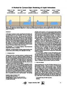
Abstract This paper extends the traditional pin-hole camera projection geometry, used in computer graphics, to a m o r e realistic camera model which approximates the effects of a lens and an aperture function o f an actual camera. This model allows the generation of synthetic images which have a depth o f field, can be focused on an arbitrary plane, and also permits selective modeling o f certain optical characteristics of a lens. The model can be expanded to include motion blur and special effect filters. These capabilities provide additional tools for highlighting important areas of a scene and for portraying certain physical characteristics of an object in an image.
In the past few years several algorithms have been developed for realistic rendering o f complex threedimensional scenes on raster displays [1,2,3]. These algorithms have been generically called hidden surface algorithms in the sense they display only the visible surfaces from a given vantage point. All these algorithms, however, have continued to use the pin-hole camera projection geometry which was developed for display of 3D line drawings on vector devices. The purpose of this paper is to develop a more complex camera model, which although computationally more expensive, provides the means of generating more realistic synthetic images closely approximating a scene imaged by an actual camera. These synthesized images are suitable for display only on raster devices. The purpose o f generating such synthetic images, which in a sense incorporate the constraints o f an optical system and the imaging medium, is twofold:
Key Words and Phrases: computer graphics, visible surface algorithms, raster displays, camera model, lens and aperture
1. It gives the ability to capture the viewers' attention to a particular segment of the image, that is, it allows selective highlighting either through focusing or some optical effects.
CR category: 8.2
2. It permits adaptation of many commonly used cinematographic techniques for animated sequences, such as fade in, fade out, uniform defocusing of a scene, depth of field, lens distortions and filtering. It should be stated, however, that the objective is to model only those features which can be used to some advantage for special effects. No attempt will be made to model flaws inherent in a lens such as optical aberrations or the lens transfer function. We will also assume that the imaging m e d i u m is perfect, that is, a point is reproduced with perfect fidelity.
*Present address: Bell Laboratories, Holmdel, NJ 07733 **Present address: Schlumberger-Doll Research, Ridgefield, CT 06877
The image generation process described here consists o f two stages. In the first stage, a hidden-surface processor generates point samples of intensity in the image using a geometric pin-hole camera model. Each sample consists of image plane coordinates, RGB intensities, z depth distance and identification of the visible surface. In the second stage, a post-processor converts the sampled points into an actual raster image. Each sampled point is converted into a circle of
Permission to copy without fee all or part of this material is granted provided that the copies are not made or distributed for direct commercial advantage, the ACM copyright notice and the title of the publication and its date appear, and notice is given that copying is by permission of the Association for Computing Machinery. To copy otherwise, or to republish, requires a fee and/or specificpermission. ©1981 ACM O-8971-045-1/81-0800-0297
$00.75
297
Computer Graphics
Volume 15, Number 3
confusion whose size and intensity distribution are determined by the z-depth of the visible surface and the characteristics of the lens and aperture model. The intensity of a pixel is computed by summing the intensity distributions of the overlapping circles of confusion of all sample points. A circle of confusion and its intensity distribution may be stretched in the image along the projected path of a moving surface to approximate motion blur caused by a finite exposure time. Special effect filters such as star or diffraction filters may be convolved with the image at this stage.
August 1981
2.2 The Finite Aperture Camera Model The basic law governing image formation through a lens can be described by the lens formula used in ray optics: ±
+ ±
U
v
_ !
(])
F
where U is the object distance, V is the image distance and F the focal length of the lens all measured along the optical axis [Figure 2]. We add to this basic lens model an aperture function which limits the lens diameter and fixes the location of the image plane at the focal plane of the lens. The introduction of these two constraints allows the notion of focusing the lens (by moving it relative to the fixed image plane), and associated with it, a depth of field. It should be stated that the notion of depth of field, that is, some objects appearing to be in focus while others are out of focus, is not a function of the optics but rather a function of the resolving capability of the human eye and the imaging medium.
2.0 T h e C a m e r a M o d e l 2.1 Camera Geometry This section describes the camera geometry used in projecting a 3D scene onto an image plane. The projection matrix, also called the camera transformation matrix, is a function of the camera parameters. These parameters are the pan, tilt and swing angles of the camera, the location of the camera lens, the focal length and the size of the image frame, as illustrated in Figure 1.
~
z1
ge plane
optical
axis
F
~Y
/
1"6"
1
~i2
\ x3
Z
xI
:~
U
:~
V
Fig. 2 Lens Law
2
\\ O3
image plane
"~-~ I " |
We will assume the accepted standard that for a viewing distance U, the smallest resolvable patch by the human eye has a diameter of U/1000. This means that anything larger than this diameter is viewed as an area (patch) rather than as a point. Alternatively, one could say that the angular resolving power of the eye is 1 rail. Based on this criteria, the depth of field can be derived as follows. Assume that at distance U, we have a patch diameter U/1000 which is in focus, that is, we can resolve it as a point. This is illustrated in Figure 3. Let diameter of the patch be MN. Extending the patch in both directions, towards and away from the lens, we obtain triangles Alvin and BMN. Note that LD is the effective lens diameter, defined as the focal length divided by the aperture number (F/n). The resulting extension of the patch MN, denoted by ~" and tf', on the optical axis, [Figure 3], will also remain in focus since their respective diameters are less than U/IO00. Since AALD iS similar to AAMN and ABLD i s similar to ABMN we obtain the following two equations:
x2
sample ray ~
viewing pyramid
....
02
center of projection
Fig. 1 Camera Geometry The use of homogeneous coordinates permits modelling this transformation as a single 4x3 matrix [5,6]. This transformation provides a perspective mapping of a point from the global coordinate system Oz, in which a scene is defined, to the image plane coordinate system 0 3. The pan, tilt and swing angles specify the direction the camera is looking at, the lens center is the vantage point relative to coordinate system 01, and the focal length along with the size of the image frame specifies the viewing pyramid. Points in Ol which lie outside the viewing pyramid are clipped from the image plane.
298
U+-t]
u+
MN
LD
a~d
U-O-
tr-
MN
LD
(2)
Computer Graphics Solving for u + and u+ -
U-
u/(t
we
Volume 15, Number 3
images of these points are resolved by the eye as points and appear to be in focus.
obtain:
o (F/,) 1000 )
(3)
T h e diameter of the circle of confusion for each point in the scene, can be expressed as follows. Let V, and Vp be the image of points U and P. ~ forms a point on the image plane whereas v, projects into a circle as it converges a distance vp - v, away. Following Figure 4 we note that ALDA and ACBA are similar. Thus we have
U u/(l + (F/.) tO00 )
IF -
(4)
The following observation can now be made: 1. If U -
LD
1000F then 0 ~ -,- ** and I F -- 500F. The tl
August 1981
CB
v.
I1
FU U-¥
where r , -
v.-v,
(7)
U>F
1000F is a close approximation to the
distance
n
FD Vp - P'"F
hyperfocal distance of a lens. A lens focused at this distance yields the m a x i m u m depth of field.
S i n c e LD = F / n and solving for CB, the diameter of the circle of confusion, we obtain
2. As the effective lens diameter is decreased, by increasing the aperture n u m b e r n, the hypeffocal distance becomes smaller in magnitude yielding greater depth o f field.
UH H-O' -
(8)
L
~
mage
plane
(5)
H U
v.-Vpl . vF.
c-I
Let us denote the hyperfocal distance as H. Then if we are focused at s o m e plane U, the limits o f the depth of field is given by: U+
P> F
UH H+U
(6)
P
~
U
~
~
-
Vp--~4 V U ~
Fig. 4 Circle of Confusion
Note that as U--P, the plane of focus, the circle of confusion approaches zero. Points at infinity approach a
limiting diameter given by ,v,F ,__
F n" The diameter of
the circle of confusion is highly asymmetric as one m o v e s away from the plane of focus in the two directions along the optical axis as illustrated in Figure 5.
D+
Fig. 3 Depth o f Field
VD F C = - - - -nF n
Diameter of . Circle of Confusion
f
2.3 Image Focusing
In this section we develop a measure o f how well a point appears to be in focus on the image plane. Since t:he image plane is fixed at F, the focal length, a point that is out of focus will converge on a plane away from F, projecting onto the image plane as a circle rather than a point. This circle is called the circle o f confusion and is a measure o f how defocussed the image point is. When we are focused at s o m e image distance U, based on our earlier calculations, a U* and a I F exist which also appear to be in focus. This implies that the corresponding image points V, Y+ and w form circles on the image plane whose diameters are less than or equal to F/1000. Thus, observed from a distance F, the
i t 1 U-~U
I
1 +
Object plane in f o c u s
Distanc~ U
Fig. 5 Asymmetricity of Depth of Field
299
Computer Graphics
Volume
It is well known from physical optics, that diffraction effects due to a finite aperture size cause the image of point source to be spread over a larger area. Our objective in studying these effects is to determine the distribution of light intensity in the circle of confusion. It can be physically observed that a defocused image results in a loss of contrast. Assuming no energy loss in lens transmittance, the distribution of energy in the image must change to account for the loss of contrast. We describe here methods to determine the light intensity distribution within the circle of confusion for defocused points.
+ y0' and ,i - ~
,0 - , / ~
+ y~
ejkF U(r0) - ~
Jkro2 e ~r l-I {U(r,)}
(11)
where H is the Hankel transform (due to the radial rl
symmetry) of the aperture circ(~-2). The light intensity distribution (power spectrum) is given by
Consider the diffraction of monochromatic light by a finite circular aperture of diameter d in an infinite opaque screen [Figure 6]. As shown, the screen is planar with rectangular coordinate system (xl,y,) and the image plane is parallel to the screen, at a distance a = F (focal length), with coordinate system(xe,yo). Let the field distribution of the wave be written as a complex function
l(,o)-
[ kd212 I Jl(kdro/F) ]2 I--I 2 I 8F I kdro/F
(12)
which is the well-known Airy pattern. A cross-section of this function is shown in Figure 7 where Jx is the Bessel function of the first order. The amplitude is dependent upon the lens diameter d thus making the intensity a function of the aperture.
(9)
where A(P) and ~(P) are the amplitude and phase of the wave at position P. '1
August 1981
If the distance rot is large compared to the diameter of the aperture, the Fresnel approximation, and assuming an ideal thin lens whose transmittance is simply a phase transformation, then U(xo,y0) reduces to the Fourier transformation of the portion of field subtended by the lens aperture. Assuming a unit-amplitude, normally incident plane wave and radius coordinates
2.4 D~raction Effects
U(P) - A (P) e-~t(e)
15, N u m b e r 3
1.0
Y
xI image plane
i
/ /
-4
observation
.~,,, -3
-2
-1
1
2
3
1 4
zI=F (Focal Length) /
Fig. 7 Light Intensity Distribution Function Fig. 6 Diffraction by a Circular Aperture The derivation of the light distribution, for defocused monochromatic images of a point source by a circular aperture, was first investigated by E. Lommel in 1885. Details of this derivation, based on the HuygensFresnel principle, can be found in [8]. The results due to Lommel can be used directly with some minor changes in interpretation.
The field amplitude at point (xo,yo), using the Huygens-Fresnel principle, can be written as
U(xo,yo) -
ff
h~(xo,yo,x~,yx)U(xx,yx)axx ay,
(10)
ri
circ ( ~ 2 )
The Huygens-Fresnel integral used to determine the light intensity in the circle of confusion cannot be obtained in a closed form and must be evaluated in terms of Bessel functions. The light intensity in the circle of confusion is given as follows:
where
ho(xo.yo.xl.y,)
1 -e-eel cos(~,7ol)
J~.
rex
k - 2=/X
l(u,v) - [2l',y2(u,v) + Y,(,,,)] , o I"1 circ(-~2)" [1 2rl/d~l [ 0 otherwise
(13)
where
kd2 l e - 8F2
• el - I z~ + (Xo - x l ) ~ + (.v0 - yx)~l ~"
and V, and V, are Lommel functions. These functions
300
Computer Graphics
Volume 15, Number 3
light sources and shadows in complex 3D scenes. Planar, quadric and bicubic surfaces can be rendered by the program at the present time.
can be evaluated by a series approximation given by V,(u,y)
-
~(-I)' (_")(.+2,) J(.+2,)(~) y
August 1981
(14)
8-O
The raster image generated by this program is considered to be a grid of square pixels lying in the image plane, that is, each pixel is a finite square area of the image. The 3D scene is sampled at points which project into the pixel corners by intersecting rays from sample points, through the center of projection (focal point) and into the 3D scene [Figure 1]. The intensity of a pixel is computed by averaging the four corner samples, which is equivalent to fitting a bilinear function into the four samples and integrating this function over the area of the pixel. Antialiasing is performed by subdividing a pixel, which has a large difference in the sampled values, into 2x2 squares [Figure 8] and recursively repeating the sampling process as described in [3]. This subdivision is done only in pixels which contain sharp intensity changes in the image, typically caused by edges, silhouettes or textures.
where J(,+2,) are the Bessel functions of the n + 2s order. The variables u and v are dimensionless and specify the position of a point within the circle of confusion. They can be expressed as follows: u
-
(15)
k(_-~d_)' z 21+
V -- k'~"~ r0 -- k
-~
+ y02
(16)
Based on the expression derived by Lommel, the following observations are made: 1. At u = 0 , that is, the distribution of light intensity of a point focused on the image plane, is given by
which is the previously derived Airy pattern.
:
2. Consider a plane at object distance p which is not in focus. This implies that the image of a point on this plane will converge at some image distance Vp. if the plane s is in focus, then Vp-v, is the distance by which the plane p is out of focus. To find the intensity distribution from the resulting circle of confusion, note that z = v, - V, or U
- k ( dZ / )" ~
(r, - V,)
•
v - k - f f ro
"/" / •
/:: •
(17)
and d
/
e/,
• •
:
•
" •
image sample point L/_(at~_p~xei corner)
L_;I
.
kedge (18)
i I ~ pixel ~-'-I--~subdivisiOn
I
I
I I
t
"- .... Fig.
8 Image
Antialiasing
gives the position in the circle of confusion. 3. Note that for v-0, the light distribution at the center of the circle of confusion, we obtain
#(.,o)-i
[ sin(u/4)]l
(u/4) I *'°
The program can optionally, in addition to generating the actual raster image, save the sampled values into a separate file. Each sampled value contains the following information:
(19)
1. The x, y coordinates in 0 3, the 2D image plane coordinate system, of the sampled point,
This shows that the highly peaked light distribution of the Airy pattern obtained for points in focus reduces in amplitude until it actually becomes zero at u/4 -- ± ~ or z - +-4,rF2/kd ~. Thus, the distribution changes significantly for points out of focus resulting in lack of contrast for defocused points.
2. the red, green and blue intensity values of the 3D scene at the sampled point, 3. the z coordinate (depth) in O~, the 3D camera coordinate system, of the visible surface, and 4. the identification number of the visible surface (to be used in motion blur).
3.0 S y n t h e t i c I m a g e G e n e r a t i o n
The parameters of the geometric camera model are also saved in this file.
3.1 Hidden-Surface Processor
The image formation process consists of two stages. In the first stage, a ray-tracing hidden-surface algorithm generates point samples of light intensity in the 3D scene within the field of view of the camera model. The program uses Whitted's recursive illumination model [3] to generate images with surface-to-surface reflections, refraction in transparent surfaces, illumination by point
3.2 Focus Processor
The focus processor can generate a raster image, which is focused and has a depth of field, from the image point samples and the geometric camera model supplied by the hidden-surface processor and from given
301
Computer Graphics
Volume 15, Number 3
lens and aperture parameters. The focus processor approximates the integration process that takes place on the film plane during an exposure.
T.
We consider each intensity sample to be an independent source of light represented by a delta function with magnitude equal to the light intensity. The response of the optical system (the lens and aperture) to this delta function is an intensity distribution function on the image plane. Assuming that the intensity distribution is negligible outside the circle of confusion and that there is no energy loss in the system, the integral of the intensity distribution function over the circle of confusion is equal to the magnitude of the input delta function. The size of the circle of confusion of a point sample is computed from its z depth and the lens and aperture parameters by equation (g), the intensity distribution within this circle is computed by equation (13). The integral of the intensity distribution over the area of a pixel [Figure 9] is the contribution of the sample point to the intensity of the pixel. The sum of such contributions, from all sample points in the image, yields the intensity of the pixel. The integral of the intensity distribution is also attenuated by the square of the z depth distance of the point sample. Finally, the brightness of the images generated by the focus processor should be the same as the brightness of the source image generated by the hidden surface processor. Brightness changes in the image caused by film sensitivity, aperture setting and exposure time are not modeled here although they would be simple to add. Hence the following expression is used by the focus processor to compute pixei intensity of the three primary colors:
xmage
/
'~ ~ 'q' N f(x,,y,,~) "
=
the
final
intensity
at
pixel
/
/ Y
/
/ Y+ ~ Y
X+ AX
inte( ral f o v e r pixel area (X, X + ~ X) (Y, Y+ A Y )
Fig. 9 Integration of Intensity Distribution over a Pixel Area The focus processor computes a number of twodimensional lookup tables at equally spaced z depth coordinates between the minimum and maximum z depth sample points in the scene. Each table contains the integral of the intensity distribution function, evaluated at the given z depth by (13), divided by the square of the z depth. This value is computed at each pixel that the corresponding circle of confusion overlaps. The table entries outside of the circle of confusion are filled with zeros. The size of each table is therefore determined by the size of the circle of confusion, in pixel units, at that z depth. The processor maintains a block of four values for each pixel in the image. These values contain the numerator of equation (20), one for each primary color, the fourth value contains the denominator of equation (20), common to all primary colors. For each input sample point, the processor selects the two lookup tables nearest to the z depth of the sample. The coresponding pixel entries in the two tables are linearly interpolated into a temporary table of coeffcients for the z depth of the current sample. The center of this table is displaced to the image coordinates of the sample point and the four values of all pixels that this table overlaps are updated. After all samples have been processed, the three primary color intensities of each pixel are computed by dividing the three numerators by the common denominator.
(20)
where Q
plane
/
/
Yi
N f(x~,y,,z,)
Q(X,X+AX, Y,Y+A Y)
August 1981
area
(X,X + AX)(Y,Y + &Y) N = the n u m b e r of point samples in the image
q, = the intensity of point sample i x, -----the x coordinate of sample i in the image plane y, = the y coordinate of sample i in the image plane za --- the z depth of sample i and also
X+AX Y+A ¥ f(X,,,i,Z,)" ~X ~ '(Z~,~/(X--Xi)2+(,--)',)2)z~ dX
4.0 R e s u l t s
(21) The focus processor described in the previous section has been implemented and used to generate a number of versions, with different lens and aperture parameters, of a test image. The geometric (pin-hole) camera version of the test image, at 512x512 resolution,
with the condition that
"f l(g,'~(x--x,)2+ly-y,)2)dy
dx - l
- w - m
302
Computer Graphics generated by the hidden-surface processor is shown in Figure 10. The depicted 3D scene consists of a 100xl00xl00 mm cube with an image of a mandrill mapped on its sides, a brown sphere of 20ram radius with a texture added using Blinn's wrinkling technique [4], and a large blue background sphere which encloses the cube, the brown sphere, the camera model and the light source. The distances of the brown sphere, the cube and the background from the camera are approximately 290, 550 and 980 ram, respectively. The camera model uses a 55 mm lens and a 30x30 mm image area. The antialiasing mechanism in the hiddensurface processor subdivides each pixel, whose value is more than 25 intensity levels (in 8-bit range) different from any of its four samples, into 2x2 squares and computes the additional five samples. In the test image [Figure 10], the hidden-surface processor computed al;proximately 350,000 samples which is about 100,000 samples more than would be required at 512x512 pixel resolution without antialiasing.
Volume 15, Number 3
August 1981
gives a summary of the focused distances, the aperture settings and the depths of field in these images. From the table values and the associated images, one can observe an increase in the depth of field due to increasing aperture settings and a decrease in the depth of field due to shorter focused distances.
Figure
ll(a) ll(b) ll(c) ll(d)
Aperture
5.6 5.6 5.6 5.6
Focused distance [mm]
U+
U-
[ram]
[mm]
2000 980 550 290
2511 1089 583 299
1662 891 521 282
Depth of field [ram] 849 198 62 17
12(a) 12(b) 12(c) 12(d)
11 11 11 11
2000 980 550 290
3333 1219 618 308
1429 819 495 274
1904 400 123 34
13~) 13(b) 13(c) 13(d)
22 22 22 22
2000 980 550 290
10000 1612 705 328
1111 704 451 260
8889 908 254 68
Focal length is 55mm Lens diameter is 9.82 mm at f/5.6 5.00 mm at f/11 2.50 mm at f/22 Table 1 Summary of Lens and Aperture Parameters Used to Generate Images in Figures 11-13
The input to the focus processor consisted of intensity point samples on a uniform square grid of 1025x1025 resolution. The focus processor computed and used four sets of 73 intensity distribution tables at 10 mm depth intervals between the nearest and farthest visible point in the scene. One set each of these tables was used for samples whose relative image coordinates were (1) in a comer of a pixel, (2) at the center of a pixel, (3) in the middle of a pixel edge in the x direction and (4) in the middle of a pixel edge in the y direction. Antialiasing was computed by dividing each pixel into 2x2 squares and evaluating equation (20) in each of the four squares. The final pixel intensity value is the average of the intensity values in the four squares.
Fig. 10 Test Image Generated with Geometric Camera Model The focus processor generated the twelve images, also at 512x512 pixel resolution, in Figures 11 to 13 from samples supplied by the hidden-surface processor. In these figures, each image (a) is focused at 2000 mm (all objects in the image are out of focus), each image (b) is focused at 980 mm (the blue background), each image (c) is focused at 550 mm (the cube), and each image (d) is focused at 290 mm (the brown sphere). The four images in each figure were generated with the same aperture setting: f/5.6 in Figure 11, f / l l in Figure 12 and f/22 in Figure 13, that is the aperture was increased by 2 and 4 stops (with corresponding "increase in exposure time" to maintain a constant image brightness) in Figures 12 and 13, respectively. Table 1
5.0 S u m m a r y This paper has developed a camera model suitable for more realistic display of complex three-dimensional scenes on raster devices. The purpose of this model is to provide new techniques for selectively implementing the optical effects of a camera on synthetically generated
303
Computer Graphics
Volume 15, Number 3
August 1981
Fig. 11 (a) Focus-- 2000ram,f/5.6
Fig. 12(a) Focus=2000mm,f/ll
Fig. 13 (a) Focus = 2000ram,f/22
Fig. 11 (b) Focus=980mm,f/5.6
Fig. 12 (b) Focus = 980ram ,f/11
Fig. 13(b) Focus=980mm,f/22
Fig. 11(c) Focus-- 550ram,f/5.6
Fig. 12(c) Focus~550mm,f/ll
Fig. 13 (c) Focus = 550ram,f/22
Fig. 11 (d) Focus-- 290mm,f/5.6
Fig. 12 (d) Focus-- 290ram,f/11
Fig. 13(d) Focus = 290mm,f/22
i i
304
Computer Graphics
Volume 15, Number 3
imagery. The model has been applied to the output of a hidden-surface program to generate images focused on various planes and an associated depth of field as a function of the camera parameters. Further extensions of this work should include generation of motion blur and modeling of special effect camera filters. 6.0 A c k n o w l e d g m e n t s The research reported here was supported by the National Science Foundation, Automation, Bioengineering, and Sensing System Program, under grant ENG 79-04821, Professor Herbert Freeman, Principal Investigator. This support is gratefully acknowledged. The authors would also like to thank Schlumberger-Doll Research for the facilities made available for the preparation of this paper. 7.0 R e f e r e n c e s
1. Catmull, E., "A Subdivision Algorithm for Computer Display of Curved Surfaces', UTEC CSc-74-133, Computer Science Department, University of Utah, 1974 2. Blinn, J.F., Carpenter, L.C., Lane, J.M. and Whitted, T., "Scan Line Methods for Displaying Parametrically Defined Surfaces', CACM, 23, (1), January 1980, 23-34 3. Whitted, T., "An Improved Illumination Model for Shaded Display', CACM, 23, (6), June 1980, 343349 4. Blinn, J.F., "Simulation of Wrinkled Surfaces', Computer Graphics 12,(3), Atlanta, Ga, 286-292 5. Carlbom, I. and Paciorek, J., "Planar Geometric Projections and Viewing Transformations', Computing Surveys, 10, (4), December 1978, 465502 6. Newman, W.M. and Sproull, R.F., Principles in Interactive Computer Graphics, McGraw Hill, Inc., Hew York, 1973 7. Goodman, J.W', Introduction to Fourier Optics, McGraw Hill, Inc., New York, 1968, Chapters 4,5 8. Born, M. and Wolf, E., Principles of Optics, 3rd (revised) edition, Pergamon Press Ltd., London, 1965, Chapter 8
305
August 1981