automatic start-up of a nonlinear distillation column model of order 42. ... From an engineering perspective, the systematic design of hybrid systems to meet given ...... Low-order models for ideal multicomponent distillation processes us-.
Abstraction Based Supervisory Controller Synthesis for High Order Monotone Continuous Systems Thomas Moor1 and J¨ org Raisch2 1
2
Research School of Information Sciences and Engineering Australian National University, Canberra Lehrstuhl f¨ ur Systemtheorie technischer Prozesse Otto-von-Guericke Universit¨ at Magdeburg, and Systems and Control Theory Group Max-Planck-Institut f¨ ur Dynamik komplexer technischer Systeme Magdeburg, Germany
Abstract. Abstraction based approaches to hybrid control systems synthesis have so far been mostly limited to problems with low-order linear continuous dynamics. In this paper, results from the theory of monotone dynamical systems are used to efficiently compute discrete abstractions for a class of nonlinear models. Furthermore, a situation is investigated where the high-dimensional plant state converges to a low-dimensional manifold; in the proposed approach the computational effort is governed by the dimension of the low-order manifold without neglecting the highorder dynamics. Results are applied to synthesize a discrete event controller for the automatic start-up of a nonlinear distillation column model of order 42.
1
Introduction
The control of a physical, biological or chemical process by a digital computer program often leads to heterogeneous systems that include both continuous and discrete event dynamics. Such systems are referred to as hybrid control systems and, in general, exhibit highly complex behaviours. From an engineering perspective, the systematic design of hybrid systems to meet given performance specifications is of particular interest; e.g. [1– 3,10,12,13,38]. When investigating suitable methodologies for particular design objectives and system classes, the development of synthesis procedures that are both efficient and reliable represents a major challenge. The demand for reliability results from safety critical applications, such as air traffic control or the control of chemical processes. As it is only for extremely restrictive conditions that hybrid controller synthesis problems can be solved directly on the basis of a hybrid plant model, a common approach is to resort to approximation based methods; e.g. [2,10–12,18,23,32]. In this context, reliability becomes a nontrivial issue: does a controller which has been synthesized for a particular approximation also achieve the design objectives for the original problem? Roughly speaking, an affirmative answer can be given under the
2
Thomas Moor and J¨ org Raisch
condition that the approximation accounts for all signals on which the original plant can possibly evolve. An approximation that exhibits this crucial behavioural inclusion property is referred to as an abstraction. This paper specifically addresses the synthesis of discrete event controllers for continuous plants with discrete external signals. For this class of synthesis problems we have developed an abstraction scheme of particular convenience, namely l-complete approximation. While for all parameter values l ∈ N0 the behavioural inclusion property is fulfilled, it can be seen that increasing l corresponds to improving the approximation accuracy. The latter is an essential feature as it allows to systematically adjust the approximation accuracy to the application at hand. By construction, any l-complete approximation can be realized by a finite automaton. Hence, the hybrid synthesis problem is transformed into a purely discrete problem, which can subsequently be solved using methods from DES theory. Some further detail on l-complete approximation in the context of supervisory controller synthesis is given in Section 2; for a self contained development of the topic the reader is referred to [18,22,32]. Our work on abstraction based supervisory control and related topics in hybrid control theory was partly funded by Deutsche Forschungsgemeinschaft under the KONDISK-scheme (research grants Ra 516/3-1, Fr 598/6-1, Fr 598/6-2, and Fr 598/6-3). This support is gratefully acknowledged. Beside our core contribution to abstraction based supervisory control [11,14,15,18,21,22,24– 26,31,32], we have also addressed hierarchical [20,27–29] and modular [16,19] extensions to our approach. We have discussed computational procedures for linear dynamics under time-driven and event-driven sampling [4,17,31] and applied our results in a number of case studies [6–9,30]. In principle, the computational procedure to generate l-complete approximations is straightforward. There are, however, two major problems that have limited applications to a class of plant models that appears small when compared to the generality of the theoretical framework provided by [18]: (i) quantization cells have to be tracked under the progress of time and intersected with other quantization cells. Clearly, this is a difficult problem if the right hand side of the differential or difference equation is nonlinear in the continuous state variable. (ii) Computational effort “explodes” with growing state dimension. Hence, applications have been restricted to fairly low-dimensional plant models. From a more general perspective, both limitations are closely related to the absence of efficient procedures for high-order and/or nonlinear reachability analysis and, in principle, also apply to other approximation based synthesis methods. In this contribution, we derive conditions for high order nonlinear systems that allow efficient computation of l-complete approximations without sacrificing reliability in the subsequent controller design. The paper is organized as follows: in Section 2, we briefly summarize the considered controller synthesis problem and the basic procedure for lcomplete approximation. In Section 3, we introduce the notion of monotone
Supervisory Control of High Order Monotone Continuous Systems
3
dynamical systems and show why it is extremely helpful for computing discrete abstractions for a certain class of nonlinear systems. In Section 4, we explore a situation that allows treatment of high-dimensional systems. Finally, in Section 5, we apply our results to synthesize a DES controller for the start-up of a distillation column that is described by a nonlinear model of order 42.
2
Abstraction based supervisory control
In our earlier work [18,22,31,32], we combine techniques from J.C. Willems’ behavioural systems theory [36,37] and P.J. Ramadge and W.M. Wonham’s supervisory control theory [33,34] to address the problem of supervisory controller synthesis for a fairly general class of hybrid systems and to establish an abstraction based solution procedure. The purpose of this section is to briefly summarize the consequences of [18,22] for the more specific case of sampled continuous systems with discrete-valued inputs and outputs; it is this class of plants that we will develop efficient abstraction procedures for in the following sections. While we need to provide an unambiguous framework for the abstraction step, technical aspects of the controller synthesis step are omitted and only an informal outline is given. For a detailed discussion, the reader is referred to [18,22]. Plant model. Consider the plant x(k + 1) = F (x(k), u(k))
and
y(k) ∈ G(x(k)) ,
(1)
where • the input signal u : N0 → U is a sequence of input symbols from the finite input alphabet U , |U | ∈ N; 1 • the state trajectory x : N0 → Rn is a sequence of real-valued states; • the state transition map F : Rn × U → Rn uniquely determines the successor state from the current state and the current input symbol; • the measurement map G : Rn → 2Y \ {∅} models a quantized measurement of the continuous state; it is not required to be deterministic. • the output signal y : N0 → Y is a sequence of measurement symbols from the finite output alphabet Y , |Y | ∈ N. This class of plant models includes a scenario of particular application relevance, namely sampled continuous dynamics with a discrete-valued input switching between a finite number of operation modes and a discrete-valued output being generated by measurement quantisation. Assuming a constant sampling period ∆ > 0, the state transition map is given by F (ξ, µ) := Φµ∆ (ξ) , 1
(2)
We denote the positive integers N and the non-negative integers N0 . We use |A| ∈ N to indicate that A is a nonempty finite set.
4
Thomas Moor and J¨ org Raisch
where for each µ ∈ U the map Φµt : Rn → Rn , t ∈ R+ 0 , denotes the flow induced by a vector field fµ : Rn → Rn ; i.e. z(t) = Φµt (z0 ) solves the ODE z(t) ˙ = fµ (z(t))
(3)
for the initial condition z(0) = z0 , and we assume unique existence of such a solution on the entire time axis. Note that if we were concerned with the system behaviour between given sampling instants, we could adopt our setup to the case of event-driven sampling. In the latter case, the occurrence of events is entirely determined by the system (e.g., by elements of the continuous state vector z crossing certain thresholds) instead of being restricted to a fixed time grid. For linear dynamics, this case has been addressed in [4,14,17]. By allowing the measurement map G to be nondeterministic, the quantization cells G−1 (νj ) ⊆ Rn , νj ∈ Y , j = 1, . . . |Y |, may cover (instead of partition) the continuous state space. This models the practically important case where measurement information is, to a certain extent, ambiguous. Supervisory control. From the perspective of a potential controller, the system exhibits a discrete event behaviour: at the k-th sampling instant, the supervisor applies an input symbol u(k) ∈ U and then waits for the next measurement symbol y(k + 1) ∈ Y . Naturally, for the problem of controller synthesis, this external behaviour plays a key role. We formally define the external behaviour B induced by (1) as B := {(u, y) : N0 → U × Y | ∃ x : N0 → Rn : Eq. (1) holds for all k ∈ N0 } ; (4) i.e. B denotes the set of all pairs of input and output signals on which the plant model (1) can possibly evolve. This definition is consistent with J.C. Willems’ behavioural systems theory, where a dynamical system is characterized by the set of trajectories that are compatible with the phenomenon it models. Following the concepts of Ramadge and Wonham’s supervisory control theory for DESs, the task of a supervisor is to restrict the plant behaviour B ⊆ (U × Y )N0 such that the closed loop is guaranteed to exhibit only acceptable signals. This specification can be formally represented by the set of acceptable external signals, denoted Bspec ⊆ (U × Y )N0 . Similar to the plant, the supervisor is characterized by a behaviour Bsup ⊆ (U × Y )N0 , which denotes the set of external signals it can evolve on. The closed-loop behaviour is the intersection Bcl = B ∩ Bsup , i.e. only those pairs of input and output signals “survive closing the loop” that are consistent with both plant and controller dynamics. The supervisor Bsup is said to enforce the specification Bspec if Bcl ⊆ Bspec . However, when interconnecting plant and supervisor one needs to ensure that the supervisor respects the input-output structure of the plant; i.e. the supervisor may enable or disable certain input
Supervisory Control of High Order Monotone Continuous Systems
5
events at any time but no restrictions must be imposed on the plant outputs. If the latter condition holds, Bsup is said to be admissible w.r.t. B; see [18] for a formal definition of admissibility. The problem of supervisory controller synthesis can then be stated as follows: Given a plant behaviour B and a specification Bspec , a supervisor Bsup is said to be a solution to the supervisory control problem (B, Bspec ) if (i) Bsup is admissible w.r.t. B, and (ii) Bsup enforces the specification. Discrete abstractions. Suppose both B and Bspec were realized by finite automata. Not surprisingly, the controller synthesis problem could then be treated by a slightly modified version of known methods from DES theory; e.g. [34]. For this case, efficient procedures are known which either compute a finite automaton realization of a solution Bsup or find that no such solution exists. However, the plant (1) is defined on the continuous state space Rn , and a finite automaton realization of B can only exist if Rn can be decomposed by a finite partition into sets of states that are indistinguishable under all external signals. This is a very restrictive condition and, in general, we can not assume that B is realizable by a finite automaton. A method to overcome this problem is to first construct a finite automaton that approximates the hybrid plant and then to solve the synthesis problem for the approximation. Various variants of this approach have been discussed, e.g., in [2,10,12,23,31,32]. In [18,22], we justify this approximation based approach by providing a sufficient condition for a solution obtained at the approximation level to remain valid for the actual hybrid plant: Consider a plant approximation Bca ⊆ (U × Y )N0 , a specification Bspec , and a solution Bsup of the supervisory control problem (Bca , Bspec ). Assume that each behaviour Bca , Bspec , Bsup is realized by a finite automaton. If Bca ⊇ B, then Bsup also solves (B, Bspec ), where B denotes the external behaviour of the plant model (1). See [18], Theorem 25, and [22], Section 6. Note that the nontriviality of this result is due to the requirement that any solution Bsup respects the input output structure of B. A plant approximation Bca is said to be a discrete abstraction of B, if (i) the behavioural inclusion Bca ⊇ B is fulfilled, and (ii) Bca is realizable by a finite automaton. The supervisory controller synthesis problem has thus been reduced to the construction of a discrete abstraction Bca ⊇ B that is sufficiently accurate such that (Bca , Bspec ) is solvable. l-Complete approximation. In the case of time invariant systems, a particularly suitable discrete abstraction is the so called strongest l-complete approximation Bl ⊇ B, where l ∈ N is a parameter. Formally, Bl can be characterized by (5) Bl := {(u, y) : N0 → U × Y | (u, y) [k,k+l] ∈ B [0,l] ∀ k ∈ N0 } ,
6
Thomas Moor and J¨ org Raisch
where the restriction operator ( · )|[k,k+l] : (U × Y )N0 → (U × Y )(l+1) picks the finite string ranging from the k-th to the (k + l)-th pair of external events and discards its absolute location on the time axis: (u, y)|[k,k+l] := [ (u(k), y(k)), . . . (u(k + l), y(k + l)) ] ∈ (U × Y )(l+1) . (6) It can be naturally extended to sets of signals: B|[0,l] := {(u, y) [0,l] ∈ (U × Y )(l+1) | (u, y) ∈ B} .
(7)
Note that B|[0,l] is a finite set as both U and Y are finite. The most relevant features of the strongest l-complete approximation Bl are that (i) accuracy is monotone in l, i.e. Bl ⊇ Bl+1 ⊇ B, and that (ii) a finite realization can be easily derived from the restricted plant behaviour B|[0,l] ; see [18], Corollary 11. Hence, there is no need to evaluate Eq. (5) in order to construct Bl . All that remains to be done is the computation of B|[0,l] and we recall the following iterative procedure from [18]: Theorem 1. Let B ⊆ (U × Y )N0 denote the external behaviour of (1). For (u, y) ∈ (U × Y )N0 and l ∈ N0 , iteratively define the sets of states X ((u, y)|[0,l] ) ⊆ Rn that are compatible with the strings (u, y)|[0,l] : X ((u, y) [0,0] ) := G−1 (y(0)) , (8a) X ((u, y) [0,λ+1] ) := F (X ((u, y) [0,λ] ), u(λ)) ∩ G−1 (y(λ + 1)) , (8b)
for λ = 0, . . . l − 1. Then, (u, y) [0,l] ∈ B [0,l] ⇐⇒
X ((u, y)|[0,l] ) 6= ∅ .
(9)
According to the above theorem, B|[0,l] can be established via a finite iteration of images under F and intersections with the quantization cells G−1 . Then, the methods presented in [18,22] allow the construction of a discrete abstraction of the hybrid plant and finally the synthesis of a supervisory controller. While this approach has been successfully applied to a number of examples, there are two major limitations from a practical point of view. First, for nonlinear continuous dynamics, images of sets of states under F can, in general, not be computed efficiently. Roughly speaking, one is often left with the simulation of an exhaustive number of initial conditions ξ0 = x(0); it is then naively assumed that X ((u, y)|[0,l] ) = ∅ whenever no ξ0 ∈ X ((u, y)|[0,l] ) can be found. Clearly, this implies the risk of omitting a particular string from B|[0,l] , hence from Bca = Bl , therefore violating the requirement Bca ⊇ B. Second, for high dimensional continuous dynamics, a reasonably accurate quantization leads to computationally intractable output alphabets Y . In the following two sections, we identify a broad class of hybrid systems where the above iterative procedure can be refined in order to gain substantial computational efficiency.
Supervisory Control of High Order Monotone Continuous Systems
3
7
Discrete abstractions for monotone systems
For monotone dynamical systems (see [35] for a comprehensive treatment of the subject), it is possible to efficiently estimate the sets of compatible states X ((u, y)|[0,l] ) and to derive a discrete abstraction from those estimates. In general, monotonicity is defined with respect to an arbitrary partial order. In this paper, we consider the specific partial order 4 which, for a, b ∈ Rn , is defined by a4b
:⇐⇒
∀ i ∈ {1, . . . n} : ai ≤ bi .
(10)
Hence, a 4 b if and only if b − a lies in the nonnegative convex cone Rn+ := {ξ ∈ R|ξ ≥ 0}n . Definition 1. The map g : Rq → Rn is called order preserving if a 4 b implies g(a) 4 g(b). Note that a map is order preserving if all its partial derivatives are nonnegative. The image of a box Q(a, b) := {c| a 4 c 4 b}
(11)
under an order preserving map g can be efficiently over-approximated via the images of a and b, i.e. g(Q(a, b)) ⊆ Q(g(a), g(b)). It is this property that allows efficient approximation of monotone systems. In the following, we consider dynamical systems z(t) ˙ = f (z(t))
(12)
and assume that, for any initial condition z(0) = z0 , there exists a unique solution Φt (z0 ) for all t ≥ 0. The dynamical system (12) is called monotone, if ordered states remain ordered under the progress of time: Definition 2. The dynamical system (12) is monotone, if the flow Φt : Rn → Rn induced by the vector field f : Rn → Rn is order preserving for all t ≥ 0. A monotonicity test can be stated in terms of the off-diagonal entries of the Jacobian of f : Theorem 2. (see e.g. [35]) The dynamical system z˙ = f (z) is monotone if ∂fi ≥0 ∂zj
∀i 6= j .
(13)
As an example, consider a linear system z(t) ˙ = A z(t). If all eigenvalues of A lie in R, then there exists a real linear transformation that transforms A in its Jordan normal form. Clearly, the transformed system is monotone by Theorem 2. For further illustration, Figure 1 shows two state trajectories z(t) � and zˆ(t) of the monotone system z(t) ˙ = −10 −11 z(t). For the respective initial
8
Thomas Moor and J¨ org Raisch
conditions z(0) = (0, −1.2)| and zˆ(0) = (0.2, −1)| we have z(0) 4 zˆ(0), and hence, by monotonicity, z(t) 4 zˆ(t) for all t ≥ 0. This is confirmed by Figure 1, which also clarifies that monotonicity of a dynamical system must not be confused with monotonicity of individual components of state trajectories: in the example, z1 (t) and zˆ1 (t) clearly fail to be monotonously increasing (or decreasing) as functions of t.
zˆ1 (t) z1 (t)
00
-0.5 −0.5
zˆ2 (t) z2 (t)
-1 −1 0
11
22
t-axis3
Fig. 1. State trajectories of a linear monotone system.
In consequence, for monotone systems, there is no need to integrate a huge number of states. Instead, the temporal evolution of a box Q(ζa , ζb ) can be over-approximated by evaluating the flow for the two points ζa , ζb only: Φt (Q(ζa , ζb )) ⊆ Q(Φt (ζa ), Φt (ζb )). Clearly, this is independent of the state dimension. We now turn to the discrete abstraction of the hybrid plant model (1), with sampled continuous dynamics (3). Obviously, during each sampling interval, the continuous dynamics depends on a fixed control symbol µ ∈ U . Under the assumption that the continuous system (3) is monotone for each µ ∈ U , it immediately follows that the transition function F ( · , µ) defined in Eq. (2) is order preserving. We further assume that measurement symbols νj , j = 1, . . . , p, correspond to bounded boxes in Rn , i.e. G−1 (νj ) = Q(aj , bj ),
a j , bj ∈ R n , a j 4 b j .
(14)
Obviously, a finite number of bounded boxes (14) can not cover the entire Rn . Hence, we need an additional out of range symbol ‡ with [ G−1 (‡) = Rn \ G−1 (νj ) , to give Y = {ν1 , . . . , νp } ∪ {‡} . (15) 1≤j≤p
Based on the iteration (8a), (8b), we are now in a position to provide easily computable conservative estimates Xˆ ((u, y)|[0,l] ) ⊆ Rn for the sets of compatible states. Using Fˆ (Q(a, b), µ) := Q(F (a, µ), F (b, µ)) as an overapproximation of the continuous evolution of a box Q(a, b) under the order preserving flow Φµ∆ , we define:
Supervisory Control of High Order Monotone Continuous Systems
• if y(0) = νj 6= ‡ for some j, let Xˆ ((u, y) [0,0] ) := G−1 (νj ) ; • if y(0) = ‡, let Xˆ ((u, y) [0,0] ) := Rn .
9
(16)
(17)
And, for λ = 0, . . . l − 1:
• if y(λ + 1) 6= ‡ and Xˆ ((u, y) [0,λ] ) 6= Rn , let
Xˆ ((u, y) [0,λ+1] ) := Fˆ (Xˆ ((u, y) [0,λ] ), u(λ)) ∩ G−1 (y(λ + 1)) ;
(18)
• if y(λ + 1) 6= ‡ and Xˆ ((u, y) [0,λ] ) = Rn , let Xˆ ((u, y) [0,λ+1] ) := G−1 (y(λ + 1)) ;
(19)
• if y(λ + 1) = ‡ and Xˆ ((u, y) [0,λ] ) 6= Rn and Fˆ (Xˆ ((u, y) [0,λ] ), u(λ)) 6⊆ ∪1≤j≤p G−1 (νj ), let Xˆ ((u, y) [0,λ+1] ) := Fˆ (Xˆ ((u, y) [0,λ] ), u(λ)) ;
(20)
• if y(λ + 1) = ‡ and Xˆ ((u, y) [0,λ] ) 6= Rn and Fˆ (Xˆ ((u, y) [0,λ] ), u(λ)) ⊆ ∪1≤j≤p G−1 (νj ), let Xˆ ((u, y) [0,λ+1] ) := ∅ ;
(21)
• if y(λ + 1) = ‡ and Xˆ ((u, y) [0,λ] ) = Rn , let Xˆ ((u, y) [0,λ+1] ) := Rn .
(22)
Note that (16)–(22) iteratively define the sets Xˆ ((u, y)|[0,l] ) for all external signals (u, y) ∈ (U × Y )N0 and for all l ∈ N0 : Eqs. (16) and (17) define Xˆ((u, y)|[0,0] ) while Eqs. (18)–(22) systematically define Xˆ ((u, y)|[0,λ+1] ) in terms of Xˆ ((u, y)|[0,λ] ). Note also that Fˆ is only applied to bounded boxes. By construction, the sets Xˆ((u, y)|[0,l] ) are guaranteed to be supersets of the sets of compatible states X ((u, y)|[0,l] ). Formally: Proposition 1. Assume that for each µ ∈ U the state transition map F ( · , µ) is order preserving and the output map G is defined by (14)–(15). Then, for all external signals (u, y) ∈ (U × Y )N0 and for all l ∈ N0 the following inclusion holds: (23) Xˆ ((u, y) [0,l] ) ⊇ X ((u, y) [0,l] ) .
10
Thomas Moor and J¨ org Raisch
Proof. Pick an arbitrary external signal (u, y) ∈ (U × Y )N0 . For l = 0 the claim follows immediately from (16) and (17). For l 6= 0, the proof is by induction w.r.t. λ = 0, . . . l −1: we assume Xˆ ((u, y)|[0,λ] ) ⊇ X ((u, y)|[0,λ] ) and show in each of the cases corresponding to Eqs. (18)–(22) that Xˆ ((u, y)|[0,λ+1] ) ⊇ X ((u, y)|[0,λ+1] ). First, observe that for the cases (19) and (22) the inclusion Xˆ((u, y)|[0,λ+1] ) ⊇ X ((u, y)|[0,λ+1] ) follows immediately. For the remaining cases, note that, by monotonicity, Fˆ (Q(a, b), µ) ⊇ F (Q(a, b), µ) holds for any a, b ∈ Rn , µ ∈ U . Hence, Fˆ (Xˆ ((u, y)|[0,λ] , u(λ)) ⊇ F (X ((u, y)|[0,λ] , u(λ)). For the case (18) one obtains Xˆ ((u, y)|[0,λ+1] ) ⊇ F (X ((u, y)|[0,λ] ), u(λ)) ∩ G−1 (y(λ+1)) = X ((u, y)|[0,λ+1] ). The same argument resolves case (20). Only case (21) remains. From condition Fˆ (Xˆ ((u, y)|[0,λ] ), u(λ)) ⊆ ∪1≤j≤p G−1 (νj ) one obtaines F (X ((u, y)|[0,λ] ), u(λ)) ⊆ ∪1≤j≤p G−1 (νj ). Together with (15), this implies F (X ((u, y)|[0,λ] ), u(λ))∩G−1 (‡) = ∅, and, hence, X ((u, y)|[0,λ+1] ) = ∅ = Xˆ ((u, y)|[0,λ+1] ). Remark: The assumption of quantization boxes instead of more general (bounded) quantization sets does not imply any loss of generality: in the latter case, we would simply replace G−1 (. . .) by Q(inf G−1 (. . .), sup G−1 (. . .)) in the above iteration (16)–(22). As an immediate consequence of Proposition 1, we obtain a finite abstraction Bca . Corollary 1. Under the same hypothesis as in Proposition 1, the following inclusions hold: � ˆ B := (u, y) [0,l] Xˆ ((u, y) [0,l] ) 6= ∅ ⊇ B [0,l] , (24) [0,l] ˆ ∀ k ∈ N0 } ⊇ Bl ⊇ B . (25) Bca := {(u, y)| (u, y) [k,k+l] ∈ B [0,l]
A finite realization of Bca can now be constructed manner as in the same ˆ . This comfor Bl (see [22,18]) – we merely have to replace B [0,l] by B [0,l] pletes the discrete abstraction procedure for monotone dynamical systems. Note that we do not assume linearity; our results are therefore applicable to nonlinear monotone dynamics.
4
Handling high-order dynamics
Many complex technical processes, although intrinsically high-dimensional, converge to a low-dimensional manifold within a short time. Distillation columns are a well-known example: a first principles modelling approach leads to a large number of ODEs describing the temporal evolution of concentrations on each tray of the column. When a column is operated, however, these
Supervisory Control of High Order Monotone Continuous Systems
11
concentrations stop to be arbitrary and form a concentration profile that can be described by very few parameters. This particular structure can be exploited in the following way: instead of quantizing the high-dimensional plant state space, only a well defined neighbourhood of the relevant part of the respective manifold is covered by quantization cells and hence provides measurement information; the “rest” of the state space returns the out of range symbol “‡”. For a formal treatment of this idea, let hµ : Rq → Rn , q < n,
(26)
represent a continuously differentiable parametrization of a q-dimensional manifold Mµ in Rn , i.e. Mµ = hµ (Rq ). Naturally, both the manifold and its parametrization may depend on the control symbol µ. Assume hµ to be order preserving and Mµ to be attractive, i.e. lim dist(Mµ , Φµt (z0 )) = 0 ,
t→∞
(27)
for all initial conditions z0 ∈ Rn , where dist(X, ζ) := inf{kζ − ξk | ξ ∈ X}
(28)
denotes the distance of a point ζ ∈ Rn to a set X ⊆ Rn w.r.t. some norm k · k. Let the bounded subset P ⊂ Rq represent the relevant operating range on Mµ and, for a given δ > 0, Vδ (hµ (P )) := {ζ | dist (hµ (P ), ζ) < δ}
(29)
the neighbourhood of hµ (P ) that is to be covered by quantization cells. We give an explicit formula for quantisation cells covering Vδ (hµ (P )) for the case where the operators dist( · ) and Vδ ( · ) refer to the so called weighted infinity norm; i.e. k · k := k · kβ∞ with kξkβ∞ := maxi |βi ξi | for P the weighting vector β = (β1 , . . . βn )| . Subject to the constraints βi > 0, βi /n = 1, the weights β may be chosen arbitrarily but are assumed to be fixed for the scope of this paper. Note that the closure of a neighbourhood of a bounded box w.r.t. k · kβ∞ is again a bounded box: V δ (Q(a, b)) = Q(a − δβ −1, b + δβ −1 ) ,
(30)
where β −1 := (β1−1 , . . . βn−1 )| , and V δ (X) denotes the closure of Vδ (X). The diameter of a box w.r.t. k · kβ∞ is defined by diam(Q(a, b)) := sup{kξ − ζkβ∞ | ξ, ζ ∈ Q(a, b)} = ka − bkβ∞ .
(31)
Given a finite a number of (q-dimensional) boxes covering P – they are referred to as parameter cells – we define the (n-dimensional) measurement
12
Thomas Moor and J¨ org Raisch
quantisation cells by [ P ⊆ Q(aj , bj ) =: Pˆ ⊂ Rq ,
a j , bj ∈ R q ,
(32)
1≤j≤pµ
G−1 (νjµ ) := Q(hµ (aj ) − δβ −1, hµ (bj ) + δβ −1 ) ⊂ Rn .
(33)
This is illustrated in Fig. 2, where, for simplicity, dependence on µ has been omitted and all βi are equal. Then, as required, the quantisation cells cover Vδ (hµ (P )). Furthermore, referring to a Lipschitz constant of hµ , the diameter of the parameter cells can be chosen such that the measurement quantisation cells meet a given accuracy requirement, i.e. the measurement cells do not exceed a given maximum diameter. Formally, this can be stated as follows:
n=2 hµ (P ) G−1 (ν3 )
q=1 P a2 a1
b1
G−1 (ν2 ) G−1 (‡)
b2 a3
G−1 (ν1 )
b3
Fig. 2. Quantization of neighbourhood of hµ (P ).
Proposition 2. Given the order preserving and continuously differentiable map hµ : Rq → Rn , let L > 0 denote a Lipschitz constant w.r.t. k · kβ∞ for hµ on the domain Pˆ ⊂ Rq . Then diam(G−1 (νjµ )) ≤ L diam(Q(aj , bj )) + 2δ. Let γ denote the maximum diameter of the parameter cells in the finite cover (32). Then [ G−1 (νjµ ) ⊇ Vδ (hµ (P )) . (34) V δ+γL (hµ (Pˆ )) ⊇ 1≤j≤pµ
Proof. The existence of a Lipschitz constant L is ensured by continuous differentiability of hµ and boundedness of Pˆ . As an immediate consequence, observe diam( Q(hµ (aj ), hµ (bj )) ) ≤ L diam(Q(aj , bj )). By the triangle inequality, we obtain diam(G−1 (νjµ )) ≤ L diam(Q(aj , bj )) + 2δ. To show the first of the two inclusions in Eq. (34), pick an arbitrary point ξ ∈ ∪1≤j≤pµ G−1 (νjµ ) and an integer j such that ξ ∈ V δ ( Q(hµ (aj ), hµ (bj )) ). Hence, there exists a point ζ ∈ Q(hµ (aj ), hµ (bj )) with kξ −ζkβ∞ ≤ δ. Obviously, Q(hµ (aj ), hµ (bj ))
Supervisory Control of High Order Monotone Continuous Systems
13
has a nonempty intersection with hµ (Pˆ ), and therefore dist(hµ (Pˆ ), ζ) ≤ diam( Q(hµ (aj ), hµ (bj )) ) ≤ γL. This implies dist(hµ (P ), ξ) ≤ δ +γL. Hence, ξ ∈ V δ+Lγ (hµ (P )), completing the proof of the first inclusion in Eq. (34). To show the second inclusion, take any ζ ∈ Vδ (hµ (P )). Then there exists a p ∈ P , ξ := hµ (p), such that kξ − ζkβ∞ < δ. By (32), we can find a j such that p ∈ Q(aj , bj ). As hµ is order preserving, this implies ξ = hµ (p) ∈ Q(hµ (aj ), hµ (bj )). Hence, ζ ∈ Vδ (Q(hµ (aj ), hµ (bj )), and, by (30), ζ ∈ G−1 (νjµ ). This proves the second inclusion in Eq. (34). The part of Rn not covered by any of the cells G−1 (νjµ ), j = 1, . . . pµ , µ ∈ U , again returns the out of range symbol ‡, i.e. [ G−1 (‡) := Rn \ G−1 (νjµ ) , (35) 1≤j≤pµ , µ∈U
such that the set of measurement symbols is given by [ µ Y := {ν1 , . . . , νpµµ } ∪ {‡} .
(36)
µ∈U
This concludes the construction of a measurement quantization based on lower dimensional attractive manifolds. The reduction of the number of required quantization cells is quite significant. If, for example, one was to cover a bounded subset of Rn by cells not exceeding a certain diameter % > 0, the number of required cells would be of the order O(1/%n ). By the above method, only O(|U |/%q ) cells are necessary to cover the corresponding portion of the manifolds Mµ , µ ∈ U . A discrete abstraction can again be obtained via Theorem 1 or, assuming monotonicity of the system dynamics, by Corollary 1, and a supervisor that is synthesized for the abstraction is guaranteed to enforce the specification for the original hybrid plant. While we have significantly reduced the number of cells, the dimension of each individual cell G−1 (νjµ ) is not affected and the propagation over time of each such cell is with respect to the fulldimensional dynamics. As indicated, the manifold Mµ may very well depend on the input symbol µ and Theorem 1 (or Corollary 1) still ensures the crucial inclusion Bca ⊇ B. Note that neither Theorem 1 nor Corollary 1 refer to the attractiveness of Mµ and therefore the respective statements remain true even if Mµ fails to be attractive. From the construction of the measurement quantization, however, the discrete abstraction Bca can only be expected to be reasonably accurate if changes in the input signal only occur when the state trajectory evolves within Vδ (hµ (P )). If the state trajectory does not approach Vδ (hµ (P )), the resulting abstraction will not purvey sufficient information on the underlying plant dynamics and we can not expect that a nontrivial specification can be enforced for the abstraction. Given a continuous system (3), a constructive proof for the existence of an attractive manifold Mµ , in general, is a nontrivial problem. However, in
14
Thomas Moor and J¨ org Raisch
contrast to hybrid controller synthesis, non-linear stability analysis refers exclusively to continuous dynamics and has been discussed in depth for many application relevant ODEs. In Section 5, we give an example of a chemical process that demonstrates how our hyrid controller synthesis framework benefits from a rich knowledge base regarding the non-linear process dynamics. A class of hybrid control problems for which an attractive manifold Mµ is readily known to exist occurs in hierarchical control architectures, in which a continuous plant is subject to a number of alternative low-level continuous controllers; see [20]. In this configuration, a high-level discrete input symbol ν ∈ U implements the activation of the respective low-level controller. In particular, for each µ the system (3) represents a continuous closed-loop model, which in many applications is required to exhibit stable state components by any resonable design objective. Again, the enforcement of such low-level design objectives refers to continuous dynamics only and for the solution of these control problems one can draw from the literature on non-linear control.
5
Start-up of a distillation column
We consider a distillation column in pilot plant scale which is operated at the Institut f¨ ur Systemdynamik und Regelungstechnik in Stuttgart. It is about 10m high, and consists of 40 bubble cap trays (consecutively numbered by i = 2, . . . , 41 from bottom to top), a reboiler (i = 1) and a condenser (i = 42), see Fig. 3. Feed is supplied on tray 21. Our application example is the separation of methanol and propanol. The following steps can be distinguished during conventional column start-up: initially, the column trays are partially filled with liquid mixture from the previous experimental run. Further feed is added, and the column is heated up until boiling point conditions are established in the whole column. During this start-up step, the column is operated at total reflux and reboil. At the end of this step, a single concentration front is established. The position of this front depends on the initial concentration and varies from experiment to experiment. In a second step, the feed F , and the control inputs (distillate and vapour flow rate, D and V ) are adjusted to their desired steady state values, and the initial front splits into two fronts. Then, in a third step, the two fronts move very slowly towards their steady state. We try to speed up the third step of the start-up procedure by introducing a suitable supervisory control strategy. The starting point for our approximation based controller synthesis is a continuous distillation column plant model which incorporates the following assumptions, which are well justified during the third step of the start-up: constant molar overflows, constant molar liquid holdups, negligible vapour holdups, total condenser, constant relative volatilities, a tray efficiency of one. Therefore, the model is based on material balances only and consists of one nonlinear first-order ODE for each tray, the reboiler, and the
Supervisory Control of High Order Monotone Continuous Systems
15
B51
LIC541
TI5403
P52
TI5402 TI599
41 FI502
F
TI583
D
FIC501
21 PDI503
TI501 TIC200
TIC300
TIC400
2
TI560
V
TI500
LIC540 FIC200
FIC300
EIC100
tank 1
tank 2
FI500
FIC400 P51
tank 3 waste tank
Fig. 3. Distillation column.
condenser [8]: niL x˙ i = FLi+1 xi+1 − FLi xi + FVi−1 yi−1 − FVi yi + yi = xi
α , 1 + xi (α − 1)
(
F xF 0
if i = 21 , (37a) else, (37b)
where xi and yi are the methanol mole fractions in the liquid and in the vapour on the i-th tray (i = 2, . . . , 41), in the condenser (i = 42) and the reboiler (i = 1); α = 2.867 is the relative volatility; xF = 0.32 is the methanol mole fraction in the feed; FLi denotes the liquid molar flow rate, FVi the vapour flow rate and niL the molar liquid holdup. Numerical values for the latter are given in Table 1. The table also states how FLi and FVi depend on F , D and V (feed, distillate and vapour flow rate). The feed flow rate is considered to be constant at F = 220.0[mol/h], while D and V are control inputs. For any constant D and V , the system (37a), (37b) has an attractive equilibrium x∗ (D, V ), which, for the nominal inputs D0 = 70.4[mol/h] and V0 = 188.2[mol/h], corresponds to the desired operating point x∗0 := x∗ (D0 , V0 ) of the distillation column. To speed up the process of approaching x∗0 , we look for a controller that switches between a finite number of constant input values. Considering only values V > 0, D > 0 such that F + V − D ≥ 0, monotonicity of (37a), (37b) follows from the criterion given in Theorem 2. The construction of lower dimensional manifolds Mµ , which is vital for approximation based discrete control, is based on wave propagation theory
16
Thomas Moor and J¨ org Raisch
Table 1. Flow rates and liquid holdups. i
FLi+1
FLi
FVi−1
FVi
niL [mol]
condenser
42
0
V
V
0
1.922
stripping
22-41
V −D
V −D
V
V
1.922
feed tray
21
V −D
F +V −D
V
V
1.922
rectifying
2-20
F +V −D
F +V −D
V
V
1.922
1
F +V −D
F −D
0
V
135
reboiler
[5]; it considers particular concentration profiles as waves and discusses their propagation in time and space. Each wave is of the form xi = p 1 +
p2 − p 1 , 1 + e%(i−s)
(38)
where p1 and p2 are the asymptotic values of the methanol mole fraction at the bottom and at the top of the wave, s is the so called wave position (point of inflexion) and % is the slope at s. The aspect of wave propagation theory most relevant to our discussion is that during the third startup step, the concentration profile can be represented by two waves of the type (38), one each in the stripping (1 ≤ i ≤ 21) and the rectifying section (21 < i ≤ 42). Their slopes can be approximated reasonably well by the slopes corresponding to the equilibrium x∗ (D, V ). For the nominal inputs D0 and V0 , the slopes turn out to be %s = 0.465 and %r = 0.572 for the stripping section and the rectifying section, respectively. Neglecting the effect of different inputs to the slopes, the lower dimensional manifold under construction becomes independent of the input symbol. If we further assume constant methanol mole fractions in the reboiler and condenser, x1 = 0 and x42 = 1, the asymptotic values in Eq. (38) are uniquely determined by the feed concentration x21 and the wave positions sˆs and sˆr for the stripping and rectifying section, respectively. 2 Consequently, the wave fronts of interest are parametrized by a map h : R3 → R42 mapping parameter triples (x21 , sˆs , sˆr ) to concentration profiles in the high dimensional state space. The i-th component hi of h evaluates to hi (x21 , sˆs , sˆr ) := x21 [ (1 − e(i−1)%s ) (1 + e(ˆss −1)%s ) ] × [ (1 − e20 %s ) (1 + e(i−22+ˆss )%s ) ]−1 2
(39)
We use the substitutions 22 − s → sˆs and 63 − s → sˆr for the wave positions in order to end up with an order preserving map h.
Supervisory Control of High Order Monotone Continuous Systems
17
for 1 ≤ i ≤ 21, and hi (x21 , sˆs , sˆr ) := [ x21 (e21%r − e(i−63+ˆsr )%r ) + (1 − x21 ) (e(ˆsr −21)%r − e(i−21)%r ) + e(i−42+ˆsr )%r − 1 ] × [ (e21%r − 1) (e(i−63+ˆsr )%r + 1) ]−1
(40)
for 22 ≤ i ≤ 42. Note that all partial derivatives of h are non-negative. Hence, h is order preserving. This completes the construction of M ≡ Mµ := h(R3 ). We now specify the operating range of the supervisor. For our particular setting, the equilibrium x∗0 corresponds to the parameter triple x21 ≈ 0.318, sˆs ≈ 10.7, sˆr ≈ 28.7. The bounded box of parameters P = [0.300, 0.340] × [4.0, 20.0] × [23.0, 37.0] is considered a reasonably large operation range, which we partition by p = 139 parameter cells Q(aj , bj ), 1 ≤ j ≤ p. The high dimensional measurement quantization cells are then constructed by Eq. (33) with δ = 0.002. Input symbols U = {µ1 , . . . µ9 } are chosen according to Table 2; see [8] for a detailed motivation of the particular numerical values. Table 2. Control symbols. symbol
µ1
µ2
µ3
µ4
µ5
D [mol/h]
35.8070
59.3318
82.8566
46.8782
70.4030
V [mol/h]
188.2433
158.6412
129.0391
217.8455
188.2433
µ6
µ7
µ8
µ9
D [mol/h]
93.9278
57.9494
81.4742
104.999
V [mol/h]
158.6412
247.4476
217.8455
188.2433
symbol
For each input symbol µ ∈ U , the system (37a), (37b) exhibits a unique solution and hence induces a flow Φµt . With the choice of a particular sampling interval (∆=10min), a hybrid plant model according to Sec. 2 is completely determined. As a specification, we require the supervisor to drive any initial state within X0 = Vδ (h(P )) into the target region Xf = V δ (h(Pf )) within no more than 20min, where Pf = [0.316, 0.320] × [8.5, 11.5] × [27.5, 31.0] ⊂ P . Choosing one of the quantization cells equal to Xf , this specification can be formalized by the behaviour Bspec {(u, y)| y(k) = νf ∀ k ≥ 2}, where G−1 (νf ) = Xf for some νf ∈ Y . Controller synthesis is then successfully carried out based on the estimate sets Xˆ((u, y)|[0,l] ) for l = 2. A simulation of the closed loop (consisting of 42nd order continuous plant model and DES controller) is shown in Fig. 4 For each sampling instant, one concentration
18
Thomas Moor and J¨ org Raisch
40
40
30
30
tray number [−]
tray number [−]
profile is plotted, the arrows indicate forward evolution in time and the intervals per tray indicate the target region Xf . As the sampling intervals in the closed-loop configuration are chosen to be 10min, the target region is seen to be reached within 20min. In contrast, Fig. 5 shows an open-loop simulation for the nominal input V0 and D0 . Here, one profile every 5h is plotted, and it takes an overall time of 20h to reach the target region.
20
10
20
10
methanol mole fraction [−] 0
0.2
0.4
0.6
0.8
Fig. 4. Closed-loop (∆=10min)
methanol mole fraction [−] 1
0
0.2
0.4
0.6
0.8
1
Fig. 5. Open-loop (∆=5h)
Remark: The properties employed for the construction of M are well motivated by wave propagation theory and also have been validated by simulations and experiments. It follows from the successful completion of the controller synthesis procedure, that our discrete abstraction is accurate enough for the particular purpose. While the insight from the process engineering perspective has been an essential guidance, it is important to note that the reliability of our controller does not depend on the various claims and assumptions regarding the process model: the only relevant requirement is the inclusion Bca ⊇ B, and this follows purely from the monotonicity of f as discussed in Section 3, see Corollary 1. On a decent workstation, the overall time required for the computation of both the discrete approximation and the supervisory controller is about 10min. This is a significant performance increase when compared with earlier work [6–8] on the very same scenario, but based on exhaustive simulation: there, computations took many hours. Note also the different quality of reliability: while our new approach guarantees the approximation to be conservative, exhaustive simulation may – in principle – overlook critical states.
Supervisory Control of High Order Monotone Continuous Systems
6
19
Conclusions
In this paper, we have shown how a general method for the abstraction based synthesis of discrete event controllers can be applied to a class of nonlinear high-order continuous systems, characterised by a monotonicity condition and an attractive low-dimensional manifold. In the presence of strict reliability requirements, abstraction based controller synthesis methods have been mostly restricted to low-order linear plant models and in this sense our contribution constitutes a considerable extension to the range of potential applications. Using monotonicity, the temporal evolution of quantization cells can be conveniently over-approximated even for nonlinear dynamics. This allows for the economical construction of a discrete abstraction for the nonlinear plant dynamics under investigation. Under the assumption that the plant state approaches a low-dimensional manifold, we construct an abstraction that in terms of computational effort depends only on the dimension of the attractive manifold rather than the full order of the plant dynamics. Note that both of our conditions lie completely within the domain of continuous dynamics: whether or not a plant is monotone and whether or not it exhibits an attractive manifold can be assessed by means of the classical theories. One might argue that our conditions are too restrictive for our results to be of practical relevance. This is not true, and we present a real-world example to support our claim to the contrary: based on a 42nd order nonlinear model of a pilot plant scale distillation column, we synthesize a discrete controller that speeds up the column start-up procedure. A comparison with earlier work underlines the achieved computational benefits. Acknowledgement: We’d like to thank D. Flockerzi for valuable discussions on monotone dynamical systems and A. Kienle, A. Itigin, and E. Klein for their help with the the distillation column scenario.
References 1. E. Asarin, O. Bournez, T. Dang, O. Maler, and A. Pnueli. Effective synthesis of switching controllers for linear systems. Proceedings of the IEEE, 88:1011–1025, July 2000. 2. J. E. R. Cury, B. A. Krogh, and T. Niinomi. Synthesis of supervisory controllers for hybrid systems based on approximating automata. IEEE Transactions on Automatic Control, Special issue on hybrid systems, 43:564–568, 1998. 3. J. M. Davoren and A. Nerode. Logics for hybrid systems. Proceedings of the IEEE, 88:985–1010, July 2000. 4. D. Franke, T. Moor, and J. Raisch. Discrete supervisory control of switched linear systems. at-Automatisierungstechnik, 48:9:461–467, 2000. 5. A. Kienle. Low-order models for ideal multicomponent distillation processes using nonlinear wave propagation theory. Chemical Engineering Science, 55:1817– 1828, 2000.
20
Thomas Moor and J¨ org Raisch
6. E. Klein, A. Itigin, J. Raisch, and A. Kienle. Automatic generation of switching start-up schemes for chemical processes. Proc. ESCAPE10 – 10th European Symposium on Computer Aided Process Engineering, pages 619–624, 2000. 7. E. Klein, A. Kienle, and J. Raisch. Synthesizing a supervisory control scheme for the start-up procedure of a distillation column - an approach based on approximating continuous dynamics by des models. Proc. LSS’98 - 8th IFAC Colloquium on Large Scale Systems, pages 716–721, 1998. 8. E. Klein, A. Kienle, J. Raisch, and H. Wehlan. Synthese einer Anfahrregelung f¨ ur eine Destillationskolonne auf der Grundlage einer ereignisdiskreten Approximation der kontinuierlichen Dynamik. 6. Fachtagung Entwicklung and Betrieb komplexer Automatisierungssysteme (EKA99), pages 447–464, 1999. 9. E. Klein and J. Raisch. Safety enforcement in process control systems - a batch evaporator example. In Proc. WODES’98 - International Workshop on Discrete Event Systems, Cagliari, Italy, pages 327–333. IEE, 1998. 10. X. Koutsoukos, P. J. Antsaklis, J. A. Stiver, and M. D. Lemmon. Supervisory control of hybrid systems. Proceedings of the IEEE, 88:1026–1049, July 2000. 11. G. Lichtenberg, J. Lunze, and J. Raisch. Two approaches to modeling the qualitative behaviour of dynamic systems. at-Automatisierungstechnik, 47:187– 198, 1999. 12. J. Lunze, B. Nixdorf, and H. Richter. Hybrid modelling of continuous-variable systems with application to supervisory control. In Proceedings of the European Control Conference 1997, 1997. 13. J. Lygeros, C. Tomlin, and S. Sastry. Controllers for reachability specifications for hybrid systems. Automatica, 35:349–370, 1999. 14. T. Moor. Event driven control of switched integrator systems. In Proc. ADPM’98 (Automatisation des Processus Mixtes: les Syst`emes Dynamiques Hybrides), pages 271–277, Reims, France, 1998. 15. T. Moor. Approximationsbasierter Entwurf diskreter Steuerungen f¨ ur gemischtwertige Regelstrecken, volume 2 of Forschungsberichte aus dem Max-PlanckInstitut f¨ ur Dynamik komplexer technischer Systeme. Shaker-Verlag, Aachen, Germany, 2000. Also PhD thesis, Fachbereich Elektrotechnik, Universit¨ at der Bundeswehr Hamburg. 16. T. Moor, J. M. Davoren, and J. Raisch. Modular supervisory control of a class of hybrid systems in a behavioural framework. In Proceedings of the European Control Conference 2001, pages 870–875, Porto, Portugal, 2001. 17. T. Moor and J. Raisch. Discrete control of switched linear systems. In Proceedings of the European Control Conference 1999, Karlsruhe, Germany, 1999. 18. T. Moor and J. Raisch. Supervisory control of hybrid systems within a behavioural framework. Systems and Control Letters, 38:157–166, 1999. 19. T. Moor and J. Raisch. Approximation of multiple switched flow systems for the purpose of control synthesis. In Proc. of the 39th International Conference on Decision and Control, CDC’00. IEEE Press, 2000. 20. T. Moor, J. Raisch, and J. M. Davoren. Computational advantages of a twolevel hybrid control architecture. In Proc. of the 40th International Conference on Decision and Control, CDC’2001, pages 358–362. IEEE Press, 2001. 21. T. Moor, J. Raisch, and S. D. O’Young. Supervisory control of hybrid systems via l-complete cpproximations. In Proc. WODES’98 - International Workshop on Discrete Event Systems, Cagliari, Italy, pages 426–431. IEE, 1998.
Supervisory Control of High Order Monotone Continuous Systems
21
22. T. Moor, J. Raisch, and S. D. O’Young. Discrete supervisory control of hybrid systems based on l-complete approximations. Journal of Discrete Event Dynamic Systems, 12:83–107, 2002. 23. P. Philips, M. Weiss, and H. A. Preisig. Control based on discrete-event models of continuous systems. In Proceedings of the European Control Conference 1999, Karlsruhe, Germany, 1999. 24. J. Raisch. A hierarchy of discrete abstractions for a hybrid plant. JESA European Journal of Automation, Special Issue on Hybrid Dynamical Systems, 32(9-10):1073–1095, 1998. 25. J. Raisch. Complex systems – simple models? In Proc. ADCHEM2000 - International Symposium on Advanced Control of Chemical Processes, Pisa, pages 275–286, 2000. 26. J. Raisch. Discrete abstractions of continuous systems - an input/output point of view. Mathematical and Computer Modelling of Dynamical Systems, 6(1):6– 29, 2000. 27. J. Raisch, A. Iitgin, and T. Moor. Hierarchical strategies for hybrid process control problems. In Proceedings of the European Control Conference 2001, pages 2534–2539, Porto, Portugal, 2001. 28. J. Raisch and A. Itigin. Synthesis of hierarchical process control systems based on sequential aggregation. In Proc. 3rd Mathmod, Vienna, pages 385–389, 2000. 29. J. Raisch, A. Itigin, and T. Moor. Hierarchical control of hybrid systems. In S. Engell, S. Kowalewski, and J. Zaytoon, editors, Proc. 4th International Conference on Automation of Mixed Processes: Dynamic Hybrid Systems, pages 67–72. Shaker Verlag, 2000. 30. J. Raisch, E. Klein, S. D. O’Young, C. Meder, and A. Itigin. Approximating automata and discrete control for continuous systems - two examples from process control. In P. Antsaklis, W. Kohn, A. Nerode, and S. Sastry, editors, Hybrid Systems V, LNCS 1567, pages 279–303. Springer-Verlag, 1998. 31. J. Raisch and S. D. O’Young. A totally ordered set of discrete abstractions for a given hybrid or continuous system. In P. Antsaklis, W. Kohn, A. Nerode, and S. Sastry, editors, Hybrid Systems IV, LNCS 1273, pages 342–360. SpringerVerlag, 1997. 32. J. Raisch and S. D. O’Young. Discrete approximation and supervisory control of continuous systems. IEEE Transactions on Automatic Control, Special issue on hybrid systems, 43:569–573, 1998. 33. P. J. Ramadge and W. M. Wonham. Supervisory control of a class of discrete event systems. SIAM J. Control and Optimization, 25:206–230, 1987. 34. P. J. Ramadge and W. M. Wonham. The control of discrete event systems. Proceedings of the IEEE, 77:81–98, 1989. 35. H.L. Smith. Monotone Dynamical Systems. American Mathematical Society, Providence, 1995. 36. J. C. Willems. Models for dynamics. Dynamics Reported, 2:172–269, 1989. 37. J. C. Willems. Paradigms and puzzles in the theory of dynamic systems. IEEE Transactions on Automatic Control, 36:258–294, 1991. 38. P.V. Zhivoglyadov and R.H. Middleton. A novel approach to systematic switching control design for a class of hybrid systems. In Proc. of the 38th International Conference on Decision and Control, CDC’99. IEEE Press, 1999.