Joint 48th IEEE Conference on Decision and Control and 28th Chinese Control Conference Shanghai, P.R. China, December 16-18, 2009
FrC14.4
Actuator Fault Estimation and Compensation based on an Augmented State Observer Approach R. J. Patton, Senior Member IEEE & S. Klinkhieo
Abstract—Faults or process failures may drastically change system behaviour leading to performance degradation and instability. The reliability and fault-tolerance of a control system can be achieved through the design of either an active or passive Fault Tolerant Control (FTC) scheme. This paper proposes a new approach to fault compensation for FTC using fault estimation by which the faults acting in a dynamical system are estimated and compensated within an adaptive control scheme with required stability and performance robustness. The FTC scheme has an augmented state observer (ASO) in the control system, which has an intrinsic robustness in terms of the stability and performance of the estimation error. The design concepts are illustrated using the notion that the friction forces in a mechanical system can be estimated and compensated to give good control performance and stability. The example given is that of a non-linear inverted pendulum with Stribeck friction.
I. INTRODUCTION
T
he reliability, robustness and fault-tolerance of the control of uncertain systems are issues that have increasing importance as modern systems grow in complexity. In keeping with these developments robust methods for detecting and isolating faults have been developed that can robustly discriminate between the effects of uncertainty and the effects of faults acting within a system or on the actuators and/or sensors. This is the subject of robust fault detection and isolation (FDI) that has been based on the use of a variety of approaches, e.g. unknown input decoupling, H∞ [1], LPV [2], sliding mode estimation [3] and non-linear geometric approaches [4]. Whilst robust FDI is concerned with the robust decision problem (detection, isolation and perhaps possible fault causes etc), the subject of FTC is concerned with the design and implementation of control schemes that are either active or passive in their method of reacting and compensating for faults [5] and [6]. During the last 12 years there has been a substantial literature on the subject of FTC as reported in the review papers[5], [6] and book [7]. FTC can be motivated by different purposes depending on the application under consideration; for example, safety in flight control, efficiency and quality improvements in industrial processes, etc. The main design challenges are: (i) the number of possible faults R. J. Patton is with the Department of Engineering, University of Hull, Hull, HU6 7RX UK (phone: +44 (0)1482-46-5117; fax: +44 (0)1482-466664; e-mail: R.J.
[email protected]). S. Klinkhieo is with the Department of Engineering, University of Hull, Hull, HU6 7RX UK (e-mail:
[email protected]).
978-1-4244-3872-3/09/$25.00 ©2009 IEEE
acting on the system and their diagnosability, (ii) the system reconfigurability in terms of available redundancy etc, and (iii) the global stability of the system. A fault can make the system deviate far from its normal operating conditions and can lead to severe change in system behaviour. Even bounded faults can cause the closed-loop system to deviate rapidly from its required operation and hence the fault accommodation time is a critical parameter. The requirement for rapid reaction to faults can mean that an FDI procedure, if used, may slow down the accommodation process. This paper is concerned with the active approach to FTC in which the controller is designed to compensate the fault effect based on on-line fault estimation. The fault estimation problem embedded within an adaptive control problem. The use of on-line compensation means that the fault isolation task is not required. The residual generation problem of fault detection is replaced by robust fault estimation. In the linear system case our control scheme makes use of observer-based output feedback. However, in the non-linear case both fault(s) and modelling uncertainties (unknown inputs) is/are estimated and compensated using an augmented state space disturbance observer structure, the ASO, with additional states corresponding to estimates of both faults and uncertainties. For clarity, this paper focuses on the special case of actuator faults within an on-line fault estimation and compensation system using the ASO concept. However, further analysis and design has shown that the approach easily handles cases of multiple faults and the co-existence of different types of faults (actuator, sensor or multiplicative faults) and unknown input signals. The controller is adaptive as the fault/uncertainty estimation signal becomes a component in the state estimate feedback control, thereby cancelling bounded uncertainty effects due to faults or unknown inputs acting on the observer state estimation error. The adaptive compensation FTC concept is illustrated by considering the friction force as a special type of input or actuator fault in a mechatronic system, the inverted pendulum. The friction (fault) estimation and compensation is handled using an Augmented State Observer (ASO) and the results demonstrate excellent performance of the adaptive controller in removing the effect of the friction force to yield very precise positioning control. To our knowledge this is the first time that friction compensation is described as a problem of FTC design for this important practical subject. Extensive recent research has focused on detailed modeling of friction phenomena in order to use robust on-line friction
8482
FrC14.4 compensation procedures [8], [9], [10] and [11]. However, the friction modeling problem remains a very difficult complex systems challenge and although complex modeling techniques are used no efficient method exists to ensure satisfactory robustness. It can easily be seen that the adaptive control approach used in this study obviates the need for explicit friction modeling. This offers significant advantages over well known model-based friction compensation methods in which detailed modeling of friction phenomena is essential and for which robustness with respect to friction characteristics is very difficult to achieve. Section II outlines the proposed approach to fault estimation and compensation using the ASO concept. The controller has two components (a) state estimate feedback together with (b) the component arising from the fault compensation. Some analysis and proof of stability for this control system structure is given, showing that the controller fault compensation gain must lie in a defined interval derived via a Lyapunov stability condition, designed via the Matlab LMI toolbox. Section III describes the results arising from the inverted pendulum friction compensation problem. Section IV provides a concluding discussion with suggestions of further research. II. AUGMENTED STATE OBSERVER The idea of estimation of uncertain effects in an observerbased FDI scheme was discussed extensively in [12], in which the uncertain effects (modeling errors, unknown disturbances etc) are combined into unknown input signals. These authors also discussed the related problem of sensitizing the FDI observer estimation error to specific faults and de-sensitising the error dynamics to other faults – effectively a dual of the unknown input de-coupling problem. This problem is also discussed in [13]. As discussed in Section I, a side-step from this is to consider a problem of fault or unknown input estimation, using robust estimation techniques. The unknown input estimation problem was considered in [12], [14] and [15] using the ASO concept and this has motivated the current FTC study. The work by Patton and Chen did not make use of fault compensation within a control loop. Here we use the ASO concept in an FTC scheme, as outlined in Section I. A. Actuator Fault estimation
actuator fault). This idea is considered even further here in the context of “an observer-based adaptive controller” of the form: (2) u = K x xˆ + K f fˆa A suitable analysis and design is required to stabilize the faulty system (1) around the origin in the presence of unwanted but bounded actuator fault signals. and K f ∈ R m×m are
K x ∈ R m×n
the controller and actuator fault
compensation gains, respectively. The vectors xˆ and fˆa are the state and actuator fault estimations signals, respectively obtained from the ASO with dynamics derived as follows:
Substitute (2) into (1), giving x& = Ax + BK x xˆ + BK
f
fˆa + Fa f a
(3)
x&ˆ = ( A + BK x ) xˆ + L x ( y − Cxˆ ) & fˆa = L f ( y − Cxˆ )
(4) (5)
Eqs. (4) and (5), can be re-arranged as: xˆ& A + BK x ˆ& = 0 f a
0 xˆ L x ( y − C xˆ ) + 0 fˆa L f ( A + BK x − L x C ) 0 xˆ L x = + y −LfC 0 fˆa L f A + BK x 0 L x xˆ L x = − [ C 0 ] ˆ + y 0 0 L f 123 f a L f 144 { 24 43 123 C x 123 ~ Ax Lx Lx x
(6) can be re-written as: ~ x& = ( A x − L x C x ) ~ x + Lx y
where Lx ∈ R
n× p
and L f ∈ R
(6)
(7) m× p
are the observer gains to
be designed [See Proposition 1 and Theorem 1 below]. The feedback gain matrix K x is obtained by linear poleplacement design by the assumption that the fault effect in the control signal will be compensated, i.e. invoking the separation principle. By solving the augmented state estimation system (7) the fault estimate f a , is obtained as the lower compatible partition of ~ x . Fig. 1 illustrates the partitioned structure according to Eqs. (1), (2) & (6).
Considering the state space representation of faulty system x& = Ax + Bu + Fa f a (1) y = Cx where x ∈ ℜ n is the state vector, y ∈ ℜ p the output observation vector, u ∈ ℜ m the input vector and A, B and C known matrices of appropriate dimensions. Fa is the fault distribution matrix for the actuator fault f a ∈ ℜ m corresponding to the ith column of B (in the case of the ith
8483
FrC14.4 Equation (1) fa
Fa
+ + +
B
1
y
C
s
(C 0 , A0 ) is observable. If the observer gains L in (11) are chosen such that there exists a s.p.d. matrix P ∈ R ( m + p ) x ( m + p ) satisfying:
A
P( A0 − LC 0 ) + ( A0 − LC 0 ) T P = −α β I where α > 0 and β ≥ f , then ~ e = [e
Equation (7) + _
Lx
a
Cx + +
1
~ x s
xˆ
M
fˆa
Equation (2)
Kx Kf
Fig. 1. ASO Fault estimation and compensation scheme Proposition 1
The estimation error system with fault corresponding to (1) and with the adaptive controller (2) and observer (4) is as follows: x& − x&ˆ = A( x − xˆ ) − LxC ( x − xˆ ) + BK f fˆa + Fa f a (8) e& = ( A − LxC )e + BK f fˆa + Fa f a
e& x A − Lx C &ˆ = Lf C f a
BK f 0
e x Fa ˆ + f a f a 0
(9)
where ex = x − xˆ ∈ Rn is the state estimation error. The closed-loop system (4) can be viewed as an interconnected system consisting of a linear observer together with a nonlinear observer whose error dynamics contain an integral action which is basically the dual of integral control. The integral term L f C in (9) will force the estimation error e x to converge to zero, and hence compensate for the actuator fault ( f a ). Since the actuator fault ( f a ) is bounded, the compensation using integral action is achievable subject to a stability condition as discussed in Theorem 1 below. Re-arranging (9) as: & ex Fa e x A BK f Lx = − [ C 0 ] fa + &ˆ 0 − L f 123 fˆa 0 f a 0 { 14243 123 C0 { { ~ e ~ F0 A0 L e&
T x
fˆaT ]T will be
contained in a bounded region around the equilibrium independent of initial conditions e x (0), xˆ (0) and f a (0) .
Ax
+ +
(12)
(10)
(10) can be re-written as: ~ (11) e& = ( A0 − LC 0 )~ e + F0 f a The closed-loop system is thus described by (4) and (11). Since the actuator fault signals ( f a ) are bounded, one can
always find a positive number β such that β > f a , where
⋅ is Euclidean norm. Theorem 1
Consider the closed-loop system described by (4) and (11) and assume that the pair ( A, B ) is controllable and the pair
Furthermore, if the controller gains K x are chosen such that the matrix A + BK x is Hurwitz then xˆ will also be contained in a bounded region around the equilibrium independent of e x (0), xˆ (0) and f a (0) , meaning that the closed-loop system (4) and (11) is stable subject to the norm bound on f a (0) , i.e. considering f a (0) as the “worst case” fault vector. This worst case follows as the appropriate region of stable attraction is defined in terms of f a (0) as defined below. Proof of Theorem 1:
Consider the following candidate Lyapunov function V = e~ T Pe~ with its derivative along the trajectories of (11): V& = ~ e T ( P( A0 − LC0 ) + ( A0 − LC0 )T P)e~ − 2~ e T PF0 f a (13) Substitution of (12) and β ≥ f a into (13) results in V& ≤ − β (α ~ e
2
−2 ~ e T PF0 )
(14)
By using the well known norm property [16]: e~T PF0 = ~ e T PF0 F0T P ~ e ≤ λmax ( PF0 F0T P) ~ e
(15)
where λmax (⋅) denotes the largest eigenvalue of (⋅) .
δ can now be defined as: 2
λmax ( PF0 F0T P ) α From (14) and (15) it follows that: V& ≤ −α β ~ e ( e~ − δ ) δ=
(16)
(17)
A region of stable attraction can now be defined as Dδ = {~ e: ~ e ≤ δ }. Following (17) it can be concluded that V& < 0 ∀ z ∉ Dδ . Therefore, there exists t 0 > 0 such that e~(t ) ∈ Dδ , ∀ t > t 0 independent of e x (0), xˆ (0) and f a (0) , hence proving the first part of Theorem 1. Since the matrix A + BK x is Hurwitz, the subsystem (4) is a stable linear system subject to inputs e x that are bounded by Dδ around the origin.
Therefore, xˆ will also be
bounded around the origin and hence the last part of Theorem 1 is proven. ■ Note that the standard linear system controllability and observability conditions guarantee the existence of the controller gain K x and observer gains L , satisfying the
8484
FrC14.4 conditions in Theorem 1. The observer gain design criterion (12) can be solved using LMI computational methods, which are widely available. The size of steady state errors is defined by the region Dδ , which can be decreased by enlarging the design parameter α , as shown in (16). Theorem 1 is also applicable for linear systems subject to unknown bounded input disturbances/faults, i.e. β is the bound of the input disturbances/faults. B. Actuator Fault Compensation Once the FDI module indicates which actuator is faulty, the fault magnitude is estimated and a new control law is added to the nominal one to avoid the fault effect on the system. Moreover, here we only consider actuator faults only one fault is assumed to occur at the same time. According to adaptive controller for compensation in (2), here is re-written as:
actuator
u = K x xˆ + K f fˆa { 123
ux
fault (18)
ua
where u x is the control of the nominal and u a is the compensating control to be added to compensate for the actuator fault ( f a ) acting in the control channels. The FTC can therefore be achieved by replacing u in (1) by (18) [see Fig. 1]. III. FRICTION COMPENSATION CASE STUDY The control of systems that involve friction in moving mechanical components presents interesting challenges [8], [9], and [10]. The tendency in recent years has been to go down a road of more and more detailed modelling of the friction phenomena in order to evoke an on-line friction compensation procedure, thereby attempting to cancel out the effect of the friction in the feedback loop [11]. FTC schemes for friction compensation can be developed which are adaptive in the sense of depending on bounded estimates of the friction forces. These requirements are satisfied when the friction force itself is considered as a fault effect. The friction force may be tolerable in the feedback system, allowing acceptable performance. However, if the system performance is degraded to a significant extent, exhibiting limit cycle oscillation, action needs to be taken either to remove the “faulty” component (e.g. replace it or giving lubricated bearing) or to invoke an automatic faulttolerant strategy in the control system. It is reasonable to consider the friction force as a fault as the friction in a mechanical system is an unwanted phenomenon in the majority of real systems [17]. This is a natural development of the modelling requirements in robust and non-linear control and estimation. Despite several important studies the friction modelling problem remains a very difficult challenge, mainly because of the
uncertain dynamic characteristics involved and that friction characteristics change over time due to, for example to wear, temperature and humidity [11]. From a control point of view, friction compensation strategies that require a detailed model of the friction characteristics have limitations arising from non-smooth non-linearity and the fact that friction modelling remains an imprecise subject, thereby resulting in a robustness problem. The friction forces acting in a mechanical system can be viewed as a specific type of actuator fault signals which act on the m control channels, whilst depending on linear velocity components (viz. as the friction forces are dependent on velocity). Hence, this is a special case of actuator fault compensation which has wide practical use in many mechanical and mechatronic systems. The practical value becomes clear from the example below, as the stability conditions are strong. Furthermore, the friction force bounds should be considered no greater than their static friction values which are often known a priori from bearing manufacturer specifications [8] and [9]. The example below shows that methods of fault estimation allied to FDI theory [10] can be used to obviate the use of very complex friction modeling, so popular currently in the control literature. Friction force estimates can be used within an FTC structure to provide on-line friction compensation. The friction estimates provide important robustness indicators for friction compensator design. Following (1), the system subject to friction forces acting in up to m of the input channels independently (e.g. on some or all of the actuated joints of a robotic system) can be rewritten as: x& = Ax + B [u − f fric ] (19) y = Cx m T represents the friction forces where f fric = [ f 1fric , K, f fric ]
acting on the system. Hence, the nonlinear friction forces that reduce the effective control forces {according to (19)} for given control inputs, can be represented as actuator faults. The proposed friction compensation methods do not require a model of the nonlinear friction forces ( f fric ). The methods only require that the friction forces should be bounded, which is a valid assumption as discussed above. To illustrate the above discussion a tutorial example of the friction compensation problem is considered using a nonlinear simulation of the inverted pendulum and cart together with simulated Stribeck friction force. The friction compensation involves estimation of a scalar friction force acting against the scalar control force u (t ) , as illustrated in Fig. 2. The cart is linked by a transmission belt to a drive wheel which is driven by a DC motor to rotate the pendulum into vertical position in the vertical plane by force control on the cart. The equations of motion including friction on the cart are
8485
FrC14.4 (M + m)&x&p + Fx x& p + m(θ&&cosθ − θ 2 sinθ ) = u(t) − f fric( x& p ), Jθ&& + Fθθ& − ml g sinθ + ml&x&p cosθ = 0
force Fs = 30 N { i.e. β < Fs = 30 }. It can be verified that
(20)
where x p , θ are the cart position and the pendulum angle, respectively. The particular values of the system parameters such as rod length and masses, etc. are given in [3].
the augmented system pair
observable. The observer gains L = [ L x
28.8285 - 2.6301 L0 = 216.3432 - 67.1367 - 1705.2120
l
θ
f fric
x p (t )
x
Pendulum Pos. [rad] Cart Pos. [m]
Fig. 2. Inverted pendulum system For simulation purposes the friction force acting on the cart is described by the discontinuous Stribeck friction model [18]: f fric = g ( x p ) Sign( x p ), xp < 0 xp = 0 xp > 0
(21)
g ( x p ) = Fc + ( Fs − Fc ) exp(− x p / v s )δ
is
the
Stribeck
linearised
system triple corresponding to the single input u (t ) and 3
measurements y ∈ ℜ .
The
three
measurements
(cart
position, pendulum angular position and cart velocity) replicate the measurements of the laboratory system. 0 1 0 0 0 1 0 0 0 , 0 0 0 1 0 , C = 0 1 0 0 A= B= 0 − 1.9333 − 1.9872 0.0091 0.3205 0 0 1 0 0 36.9771 6.2589 − 0.1738 − 1.0095
In this study, it is assumed that only the position measurement of the cart ( x p ) and the angle of the pendulum ( θ ) are available for the feedback loop, i.e. C = 1 0 0 0 . 0 1 0 0
The friction compensation gain is chosen as K f = 1 , corresponding to the bound arising from the static friction
Compensator ON
0 -0.1
0
20
40
60
80
0
20
40 Time [s]
60
80
0.1 0 -0.1
Friction Compensation Error [N]
Fc = 5 N , Fs = 1.25 N , v s = 0.15 ms −1 and δ = 1.22 A linearization of the left hand side of (21) results in the perturbation states x = [ x p , x& p , θ , θ&] corresponding to the The
Compensator OFF
0.1
Friction Forces [N]
friction levels, respectively and v s , δ > 0 are the Stribeck velocity and shaping parameters, respectively. In the simulation the following parameter values are used:
point: x p = x& p = θ& = θ = 0 .
39.0105 - 92.7549
Fig. 3. ASO friction compensation simulation results for the friction compensation activated at time t = 40s.
friction function with Fc and Fs are the Coulomb and static
equilibrium
513.3875 2119.5169
- 3.5192
K x is designed by placing the eigenvalues of ( A + BK x ) at -4.5, -6.0, -7.5 and -9.0. Simulation results for given initial values: x(0) = [1.1 − 1.1 0 0]T and f a (0) = 1 are shown in Figs. 3 and 4.
M
{−1} if where Sign( x p ) ∈ [ −1, 1] if {1} if
L f ]T are designed
The controller gain
mg P
0
as in (11) is
such that the eigenvalues of ( A0 − LC 0 ) are placed at -12, 16, -13, --15, and -14 satisfying condition (12), is given by:
y
u (t )
(C 0 , A0 )
5 Friction f fric Estimate
0
-5 50
55
60
65 Time [s]
70
75
80
55
60
65 Time [s]
70
75
80
5
0
-5 50
Fig. 4. Comparison of friction force and its estimate Fig. 3 shows that for t < 40 s the augmented state fˆ fric is switched off, illustrating that the inverted pendulum model system exhibits limit cycle oscillation around the vertical equilibrium point (the origin). This is because the cart, which is affected by the friction, exhibits stick-slip motion. For t > 40 s the compensator is activated via K f f a in (18) so that the limit cycle oscillation is significantly reduced to very a small neighbourhood around the equilibrium point as predicted by Theorem 1. After compensation the amplitude of the pendulum angular oscillation is less than 6.5 mrad and
8486
FrC14.4
the amplitude of the cart stick-slip motion is less than 6 mm. These results can be achieved since the friction force is accurately estimated by the compensation term K f f a as depicted in Fig. 4. Some spikes occur in the friction estimation/compensation error as shown in the lower part of Fig. 4, which are due to the discontinuous nature of the friction force during the transition of the stick-slip motion. This discontinuous nature of the friction cannot be followed immediately by the friction estimate. IV. CONCLUSION
ACKNOWLEDGMENT S Klinkhieo acknowledges PhD scholarship funding from the Synchrotron Light Research Institute (SLRI) under the Royal Thailand Government. REFERENCES [1]
[2] [3]
This paper proposes a new strategy for FTC making use of for fault estimation and compensation via the design of an augmented state observer (ASO) whose integrated estimation error has the effect of compensating each fault signal. The integral of the observer estimation error is represented according to an augmented system description. In this paper the additional states are shown to be estimates of actuator faults. An adaptive control fault compensation method has been developed and analyzed and the new compensating control is computed using the estimation information, derived from bounds on the faults. A tutorial example is given of the compensation of friction force in the inverted pendulum, as an FTC problem considering the friction force as an input channel (actuator) fault. It is clear from this study that the friction compensation problem for a mechanical system can be viewed as an FTC problem which does not require a model of the friction forces. It is interesting to note that although most studies consider the friction force to have an uncertain effect on the system it is more constructive here to view the friction force as a particular fault. From a practical standpoint this method can be implemented well on real-time application systems. Additionally, when compared with the model-based compensation methods the advantage gained is that the model-robustness problem is obviated and this is considered of practical significance. For the friction problem, the on-line fault estimation/compensation strategy proposed circumvents the complexity problem that can arise when model-based friction compensation methods are used. As friction phenomena are so difficult to model, the friction estimation approaches may yield better robustness and improved friction compensation. The combined fault estimation and compensation problem provides a powerful method of loop-transfer recovery, enabling the Separation Principle to be reached as the faults and/or uncertainties are estimated. Whilst the example given is an illustration based on the friction compensation problem, the theory and approach has wide application to more complex problems in which actuator, sensor faults as well as multiplicative faults and unknown input signals can all be compensated together using the system description and stability conditions of Section II. A discussion of this will be the subject of an extended study.
[4]
[5]
[6]
[7]
[8]
[9]
[10] [11]
[12] [13]
[14]
[15]
[16]
[17]
[18]
8487
J. Chen & R. J. Patton, (200), Standard H∞ filtering formulation of robust fault detection, IFAC Symposium SAFEPROCESS 2000, pp 256-261, Budapest, June 14-16. J. Bokor & G. Balas (2004), “Detection filter design for LPV systems – a geometric approach,” Automatica, Vol. 40, pp. 511-518. C. Edwards, S. K. Spurgeon & R. J. Patton (2000), “Sliding mode observers for fault detection and isolation”, Automatica, vol. 36, pp.541-553. C. DePersis & A. Isidori (2001), "A geometric approach to nonlinear fault detection and isolation", IEEE Trans. Aut. Cont, AC-Vol. 46, No. 6, pp. 853-865. R. J. Patton (1997), “Fault-tolerant control: The 1997 situation (survey)”, IFAC SAFEPROCESS’97, Hull, UK, August 26-28, 1997, Vol. 2, pp. 1033-1055. M. Blanke, M. Kinnaert, J. Lunze & Staroswiecki M, (2003), Diagnosis and Fault-Tolerant Control, Springer-Verlag. ISBN: 3540010564. M. Blanke, C. Frei, F. Kraus, R. J. Patton, M. Staroswiecki. (2000), What is Fault-tolerant control? Proc. IFAC Sympo. On Fault Detection Supervision and Safety for Tech. Pro., Budapest, Vol. 1, pp. 40-51. B. Armstrong-Hélouvry B, P. Dupont, & W. C. Canudas de, (1994), A survey of models, analysis tools, and compensation methods for the control of machines with friction., Automatica, Vol. 30, No.7, pp. 1083–1138. H. Olsson, K. J., Aström, W. G. Canudas de,M. Gäfvert & M. Lischinsky, (1998), Friction models and friction compensation, European Journal of Control, Dec. 4, pp.176-195. Armstrong B S R & Chen Q, (2008), The Z-properties chart, IEEE Control Systems Magazine, Vol. 28, No. 5, pp. 79-90. B. Bona & M. Indri, (2005), “Friction Compensation in Robotics: an Overview”, Proc. the joint 44th IEEE Conference on Decision and Control and the European Control Conference 2005, pp. 4360-4367. J. Chen & R. J. Patton, “Robust Model Based Fault Diagnosis for Dynamic Systems”, Kluwer Acad. Pub. ISBN 0-7923-841-3, 1999. F. J. Uppal & R. J. Patton, (2005), Neuro-fuzzy uncertainty decoupling: A multiple-model paradigm for fault detection and isolation, Int. Journal of Adaptive Control & Signal Processing, (Invited Special Issue Paper), Vol. 19, No. 4, pp. 281-304. R. J. Patton & J. Chen, (1992), Robust fault detection of jet engine sensor systems using eigenstructure assignment, Journal of Guidance, Control & Dynamics, 15(6), 1491-1497. J. Chen & R. J. Patton, “Optimal filtering and robust fault diagnosis of stochastic systems with unknown disturbances”, IEE Proceedings on Control Theory & Applications, vol. 143 no. 1, pp. 31-36, 1996. C. Edwards, S. K. Spurgeon & R. J. Patton, (2000), Sliding mode observers for fault detection and isolation, Automatica, Vol. 36, pp.541-553. R. J. Patton, D. Putra & S. Klinkhieo, “Friction Compensation as a Fault-Tolerant Control Problem, Semi-Plenary Paper”, 23rd IAR Workshop on Advanced Control and Diagnosis, November 27-28, 2008, Coventry University, United Kingdom. D. Putra, L. Moreau & H. Nijmeijer, “Observer-Based Compensation of Discontinuous Friction”, Proceedings of the 43rd IEEE Conference on Decision and Control, the Bahamas. pp. 4940-4945, 2004.