present a comparison of these methods on both French and English text corpora. ... improve information retrieval significantly (J.Callan, 1994), by giving the ...
Adapting and comparing linear segmentation methods for French Laurianne Sitbon , Patrice Bellot Laboratoire d’Informatique d’Avignon - Universit´e d’Avignon 339, chemin des Meinajaries - Agroparc BP 1228 84911 AVIGNON Cedex 9 - FRANCE Tl : +33 (0) 4 90 84 35 09 Fax : +33 (0) 4 90 84 35 01
{laurianne.sitbon , patrice.bellot}@lia.univ-avignon.fr
Abstract This paper presents an empirical comparison between different methods and tools for segmenting texts. After presenting segmentation tools and more specifically linear segmentation algorithms, we present a comparison of these methods on both French and English text corpora. This evalutation points out that the performance of each method heavilly relies on the topic of the documents, and the number of boundaries to be found.
1
Introduction
Segmentation task has many objectives and many algorithms have been developped to achieve it. We are interested in those which are unsupervised and which produce linear segmentations. This work is done in the context of the project ”Technolangue AGILE - OURAL” financed by the French minister of research. The implementations we tested are DotPlotting (Reynar, 2000), C99 (Choi, 2000), Segmenter (Kan et al., 1998), and Text Tiling (Hearst, 1994). They have been created for the English language, and compared in (Choi, 2000). As far as we know, a comparison of these tools has not been published on French texts. After adaptating these tools for the French language, we evaluate the performance of each of them on a French corpus. These tests show on one hand differences of performance, and on the other hand how they are affected by various factors like language, topic, text category, and the number of boundaries to be found.
2
Segmentation objectives and methods
Segmentation is a task with multiple applications and multiple methods. That is why we have to consider a specific class of tools and objectives, in order to be able to compare them. A segmentation can improve information retrieval significantly (J.Callan, 1994), by giving the specific part of a document corresponding to the request as a result, and by indexing documents more precisely : by subdividing texts into thematically coherent segments, a segmentation step allows to better estimate the relevance compared to the request. The second very popular role is represented by the task of TDT (Topic Detection and Tracking). It consists in detecting boundaries between articles in a flow of informations, broadcast news, and textual transcriptions. Finally, segmentation can be part of a summary process, for example in TXTRACTOR (McDonald and Chen, 2002). This can be used for selecting the most representative sentence of each segment and producing a summary. It can be used to indicate the most representative segment and giving it as a summary.
Word position x 103 3.00 2.80 2.60 2.40 2.20 2.00 1.80 1.60 1.40 1.20 1.00 0.80 0.60 0.40 0.20 0.00 0.00
0.50
1.00
1.50
2.00
2.50
Word position x 103 3.00
Figure 1: DotPlotting : each dot reveals the presence of a word at the coordinates place
The methods are mainly divided into two groups: those using learning corpus and those which do not. The second group can be divided in two groups: the algorithms which applies linear segmentation, by placing boundaries between segments, and those which apply clustering in topic classes on retrieved segments. This suppose that topics can be crossed and is founded on clustering text sentences, and link each cluster to a topic. This clustering can be implemented by means of similarity measure as in (Salton et al., 1996), or by means of decision trees for example.
3
Algorithms for linear segmentation
The algorithms detailed in this section are those used in our experiments. They are based on lexical cohesion (Halliday and Hasan, 1976), non supervised (domain independent ?), and they produce linear segmentation (opposite to hierarchical segmentation).
3.1
Dot Plotting: term repetition
This algorithm proposed in (Reynar, 2000) is an adaptation for text segmentation of a more general technique called dotplotting (Helfman, 1994). The principle of dot-plotting is that the positions of occurrences of terms in the text to be segmented are represented in a graph. If a term appears at both positions x and y, points (x,x), (x,y), (y,x) and (y,y) are plotted on a graph like on Figure 1. This graph lets the reader (human or machine) know which parts of the text contain many term repetitions. The adaptation proposed by (Reynar, 2000) consists in defining that begin and end positions of most dense zones of the graph are the boundaries of thematically coherent segments. The density is computed for each unit area by dividing the number of points in a region by the area of that region. Then two algorithms can be implemented using that measure. One consists in identifying the boundaries which maximize the density within segments . The other consists in locating boundadries which minimize the density of regions between segments.
Figure 2: C99 : steps of division of a document in topically coherent segments
3.2
C99 : similarity measure
This algorithm presented in (Choi, 2000) uses a similarity measure between each minimal unit (in our experiments, the minimal unit is a sentence). It is based on the idea that the similarity values of short text segments is statistically insignificant, and so only the order can be considered to apply a clustering algorithm on the similarity matrix. The first step of this method consists in constructing a similarity matrix between sentences of the text, using the cosine similarity measure defined in (Rijsbergen, 1979) : sim(x, y) =
P fx,j ×fy,j qP j P 2 , 2 j fx,j × j fy,j
where fs,w is the frequency of word w in sentence s. This is evaluated for each pair of sentences of the text, using each common word between the sentences, after removing stop words and applying a stemmer. Then a ranking is done, determining for each pair of sentences, the rank of its similarity measure compared to its n × m − 1 neighbors, n × m being the chosen ranking mask with n and m being number of sentences. The rank is the number of neighboring elements with a lower similarity value. In order to consider the side effect (less neighbors examined on the sides of the matrix), the rank is stored as a ratio r: r=
rankcalculated number of neighbors in the mask
Finally the last step imitates the preceeding dotplotting algorithm by maximization. Each tested potential repartition of m segments which are squares along the diagonal of the ranking matrix, and for each ak (area of the segment k) and sk (sum of the ranks in k are computed). Then the density of the repartition is computed by : D=
Pm k=1 sk Pm , k=1 ak
The potential repartitions are first the entire document, and then each splitting of the preceding found segments as shown in Figure 2, and so on until the best reduction of D by splitting is significantly low.
3.3
Segmenter : lexical chains
Segmenter, proposed in (Kan et al., 1998), makes a linear segmentation based on lexical chains appearing in the text. Those chains link all the occurrences of a term inside the text, some from a sentence to another. A chain is considered broken when the number of sentences or words between 2 occurrences of the word it is linked on is significantly too high. The threshold employed depends on syntactical category of the given term (indeed a proper noun is often replaced by its pronoun, so there can be a lot of sentences evocating this noun without mention it, so the threshold for this kind of terms must be higher than for others). Once all chains have been extracted, they are weighted depending on the syntactical category of the linked term, and on their length. Then each paragraph receives a score, calculated according to the weight of links it contains, and the history of those links (beginning or ending in the considered paragraph is noticeable). Thus boundaries are assigned at the beginning of the highest scored paragraphs. As one concept can be evocated by a lot of different words, lexical chains could be constructed on concepts instead of stems, based on Wordnet (Fellbaum, 1998) or other semantic network or ressources. (Kan et al., 1998) showed that it gives only minor improvement in precision. Moreover, it should add confusion as some words can belong to different concept groups.
3.4
Text Tiling : multi-criteria on terms distribution
Text Tiling algorithm (Hearst, 1994) and (Hearst, 1997) looks at terms repartition according to several criteria. A score is computed for each paragraph depending on its following paragraph. This score depends on a second score (lexical score) given to each pair of sentences according to the next pair of sentences. This last score is computed with one of the following criteria, also represented in Figure 3: • the common words (scalar product of vectors counting occurrences of each term in each pair of sentence); • the number of new words; • the number of active lexical chains (a lexical chain is told active if the link is contained in the pair of sentences analyzed). Then the similarity of each paragraph is computed with the normalized scalar product of lexical scores of each pair of sentences it contains. The boundaries are affected into segments whose similarity score is very different from the score of the preceding and the following segment. It is clear on a graph like in Figure 4 that thematic boundaries corresponds to quick variations :
4
Evaluation
This section introduces several ways of evaluating segmentation algorithms. It deals with the advantages and inconvenients of classical recall/precision, and presents two measures, Pk wich has been improved to give Window Diff, the measure we used for our experimentations.
4.1
Classical recall/precision
The two standards recall and precision, classically used in information retrieval, detailed in (Baeza-Yates and Ribeiro-Neto, 1999), were often employed to evaluate segmentation algorithms. But they are not so
7
6
5
4
Figure 3: TextTiling : finding boundaries with (a) repetition of words, (b) apparition of new words, (c) active chains 3
2
1
0 1
-1
2
3
0
4
10
5
6
7
20
8
9
30
10
11
40
12
13
50
14
15
60
16
17
70
18
19
80
20
90
100
0.6
0.5
0.4
0.3
1
2
3
4
5
6
7
8
9
10
11
12
13
14
15
16
17
18
19
20
0.2
0.1
0 0
10
20
30
40
50
60
70
Figure 4: TextTiling : interpreting scores
80
90
100
relevant for many reasons. First, they are too related to each other, and we are not looking for supporting more one or the other, but evaluating the algorithms globally. To solve this problem, (Jr. et al., 1997) proposed an other measure, the Harmonic Mean, which gives only one result, combining both recall and precision. But this is difficult to interpret as a meaningful performance measure. Another problem is that they do not weight errors because they are locally binary measures. It means that the error is the same if there is one sentence between the found boundary and the real boundary, or if there are 5 sentences. Finally, for algorithms like dot plotting where the number of boundaries to find is predefined, recall and precision are equal. This is because the number of boundaries to find (used for recall) and the number found by the algorithm (used in precision) is the same in those cases.
4.2
Beeferman measure : Pk
In order to go over those problems, (Beeferman et al., 1997) proposed an other measure that takes into account the distance (computed in number of words for example) between a boundary found and the right boundary to find. The first proposed measure was the probability for any pair of sentences to be in the same segment in the hypothetical segmentation (hyp) if they are in the same segment in the reference segmentation (ref), and to be in different segments in hyp if they are in ref. Formally that gives : P L PD (ref, hyp) = D(i, j).(δref (i, j) δref (i, j)) L where means XNOR (both or neither), and δx (i, j) is a boolean set to 1 if sentences i and j are in the same segment in segmentation x and 0 if they are in different segments. D is a distance probability distribution for each set of distances between random sentences. Then, they proposed a simplification of this measure in [Beef99], fixing the distance between the two sentences to a fixed number, which is half the average number of words in a segment. A probability of ”error” is then calculated on the segmentation : p(error — ref, hyp, k) = p(miss — ref, hyp, different ref segments, k) p(different ref segments — ref, k) + p(false alarm— ref, hyp, same ref segment, k) p(same ref segment — ref, k) An hypothesized boundary which is far from the reference one at greater a distance than k is considered as false alarm where it is and as missing where it should be (the same place as the reference one). It is also considered as 2 errors instead of 1.
4.3
Hearst measure : WindowDiff
(Pevzner and Hearst, 2002) shows that Beeferman measure, even if it is better than recall and precision, presents some failures. Five bad points have been highlighted in (Pevzner and Hearst, 2002) : • Missing boundaries are more penalized than false alarms. • When a boundary is added implying a new segments of size smaller than k, it is not detected and so not added in the score. • The algorithm is more lenient when there are strong variations in segment sizes. • Near-miss errors are penalized too much compared to false alarms and missing boundaries. • The meaning of the score is not clear : it looks like a percentage but it is not. They proposed a new way of scoring L segmentation algorithms, called Window Diff. It is almost identical to Pk , except that instead of which is evaluated to 0 or 1, they use the difference between the number of boundaries between positions i and i+k in both ref and hyp. If this difference is null so
the sentences i and i+k are locally in the same segments of ref and hyp. This let small added segment in hyp be penalized. P WindowDiff(ref, hyp) = N 1−k (|b(refi , refi+k ) − b(hypi , hypi+k )|), where b(xi , xj ) represents the number of boundaries between positions i and j in the text x, and N represents the number of sentences of the text. They experimently show that this measure is stable with variation of segment sizes and equivalent for false alarms and missing boundaries. This new measure presents the inconvenient that the score can now be greater than 1, so it can no longer be assimilated to a percentage. Thus, it is now clear that the measure is only for comparison, and does not evaluate the quality of a segmentation algorithm directly.
5
Testing on the French language
In order to use the implementations of (Choi, 2000), we had to adapt them for the French language, create a corpus, and add a new measure for evaluation purposes.
5.1 5.1.1
Language dependent modules Stopword list
A stopword list is used to filter non informative words from a text. This is necessary because as they appear very frequently, they could produce biased lexical chains or increase artificially similarity between paragraphs. The French stopword list used can be found in (Veronis, ). It is used by algorithms that do not use part of speech tagging to eliminate non informative categories of words. 5.1.2
Stemmer
Porter’s stemming algorithm (Porter, 1980) is very efficient for the English language, but is not adapted to process French. Moreover, it is not based on a parameter file with the specificity of the language. We replaced it by an implementation of Snowball (Porter, 2001) with a French parameter file given with the tool. Snowball is a language in which stemmers can be easilly defined and from which fast stemmer programs in ANSI C or Java can be generated. 5.1.3
Part-Of-Speech Tagging
The tagging process, which consists in finding syntactical categories of each word of a text, in context, is only used by the tool so-called Segmenter. Initially, a very fast client server was used, based on QTag. We replaced by Tree Tagger ((Schmid, 1994) and (Schmid, 1995)). The interpretation of a PartOf-Speech tagset is language dependent. Therefore these tags has to be converted to each Segmenter specific category tagset. This process does not depend on a parameter file, so it has to be done for every new language.
5.2
Evaluation Corpus
We manually built a corpus containing documents related to different themes (sciences, art, economics, ...). Each theme is represented by various size of segments. Topics ans size of segments are the two
dimensions used in the comparison of different methods. 5.2.1
Reference corpus
The reference corpus has been built from two sources of documents. The first one consists of randomly chosen articles (with more than 10 sentences) of the French newspaper ”Le Monde” published during 2001. The second one is made of randomly chosen chapters of the Bible. In each reference document, each segment corresponds to the beginning of a new article. Thus defined segments are different enough to be bounded accordingly to every human judges. Each document of the reference corpus is a made of 10 segments. The topic and the size of the segments is explained below. 5.2.2
Topic variation
6 subclasses of the reference corpus have been created in order to show the influence of document topics and categories in the segmentation process. They can be grouped in 3 sections : • newspaper articles on various topics; • newspaper articles on specific topics : art, economics, sciences or sport; • extracts of the Bible. These variations allow us to analyse the results according to several dimensions. We are able to compare methods depending on the kind of documents used. We can also consider the influence of the homogeneity or the heterogeneity of the corpora processed by the segmentation tools. Indeed the first newspaper corpus is heterogeneous and the four next ones can be considered as homogeneous. 5.2.3
Size variation
For each of the preceding categories, the subcorpus is made of 4 corpora of 100 documents. These 4 subcorpora are build in order to contain different segment sizes and different range of variations in the segment sizes inside a document. The size of a segment is the number of sentences contained in it. The documents of the first three subcorpora are made of segments of similar sizes : small (between 3 and 5 sentences), medium (between 6 and 8 sentences) and large (between 9 and 11 sentences). The fourth subcorpus contains documents having 10 segments of any preceeding sizes. Thus two aspects of this variation are considered : having large/small variation in size of different segments, and having large or small segments.
6
Experiments
Our experiments have been done with several goals, not only comparing the methods, but considering the impact of the document properties (category or segment size) on the segmentation performance. The fact that some algorithms can take into account a fixed number of boundaries is considered. We aim to propose new ways of using these algorithms, depending on the segmentation goals and on the properties of the documents.
Figure 5: comparison between results on french corpus and on english corpus, with Hearst measure
6.1
Validation of the French adaptation of the tools
Once the adaptation to French has been done, a comparison between French and English results is performed in order to validate these modifications. Figure 5 shows that the mean of the difference between results of tests on English corpus with original algorithms and tests on French corpus with modified algorithms is about 0,1 (according to Window Diff measure). Thus the algorithms seem to have been well adapted to French language.
6.2
Comparison between English and French results
The results on the English corpora are better than the French ones according to Figure 5. This can be explained as follows. Our French corpus is not a translation of the English corpus we used, so even if it has been built as close as the way the English one was (from articles of any categories of a newspaper corpus), it is possible that the segments of the english corpus are more consistent than the French ones, or that the thematic differences between segments in the English corpus are more important. Moreover, as the stemming tools are not the same, they might be less efficient on the French data.
6.3
Comparison of tools without prediction on the number of segments
Table 1 shows the mean Hearst measure on the whole test corpus for five different tools. This shows that C99 seems to be the most efficient method, twice as good as Text Tiling and Segmenter both using lexical chains. This shows that the java implementations of Segmenter and Text Tiling proposed as
JSegmenter C99 basic Text Tiling JTextTile Segmenter
0,78202381 0,27374675 0,53002938 0,9 0,50826998
Table 1: comparison of algorithms with unknown number of boundaries, with the mean of Hearst measure Categories Test nb score 25 4 36 4 37 4 38 4 13 3 32 3 34 3 35 3 11 1 12 1 14 1 15 1 31 1 33 1
Sizes Test nb score 25 4 35 3 36 3 37 3 34 2 38 2 32 1 33 1 38 1
Table 2: competition between algorithms with different parameters, for each category and for each size range of segments
improvements by (Choi, 2000) are less efficient in French. In our experiments Segmenter and Text Tiling are handicaped by the fact that they usually work on paragraphs as unit blocks, and here in the experimentation, paragraphs are equivalent to sentences. These results could also be considered biased by the fact that for large segments, it is possible that the part of article they are extracted from is itself composed of two or more segments.
6.4
Comparison of tools knowing the number of boundaries
In order to evaluate these tools, we construct a tournament to determine which ones are better along criteria of sizes on one hand and categories on the other hand. This is done by giving points to the 5 best tools/parameters for the best of each category/size. Here are the results for the categories (resp. sizes), where the scores represents the number of categories (resp. sizes) where the test figures in the 5 bests results. The test numbers are given in Table 5. Table 2 shows that C99 with diverses parameters is better than dotplotting when the number of boundaries is pre-fixed.
Figure 6: results of Hearst measure on algorithms tested on french corpus with various known number of boundaries
6.5
Using a range of number of boundaries
As the algorithms with predicted number of boudaries are significantly more efficient than ones without, we compute them with other number of predicted boundaries, to see if we can consider them as good in a certain range of boundaries. This range can later be considered as a granularity of segmentation. The graph in Figure 6 shows that even with an error in the number of boundaries at a half level, the best algorithms with defined n can be as good as other parameters with kown n, and better than Segmenter or Text Tiling, in this experimentation. This possibility of giving a range for the segmentation is the most user friendly as the need of segmentation can vary with usage and documents.
6.6
Efficiency by category or size
Table 3 summaries evaluation for the 3 better algorithms of each category and any size, and for each size and any category : Table 3 shows about sizes that it is harder to retrieve small segments than large ones, and that the non homogeneity of sizes is a handicap. About categories, data from litterature (the Bible in our case) are harder than other ones, and the easiest are ”general” and ”economics” data. This is probably due to the fact that the subjects are more various in the general corpus, and the proper nouns are more important and various too in economics category.
Size 3-5 3-5 3-5 6-8 6-8 6-8 3-11 3-11 3-11 9-11 9-11 9-11
H. measure 0,224491436 0,226962135 0,227098029 0,192753249 0,192794097 0,194685313 0,213174437 0,213174437 0,2178879 0,166995467 0,167225079 0,167878052
Category General General General Art Art Art Bible Bible Bible Eco. Eco. Eco. Sciences Sciences Sciences Sport Sport Sport
H. measure 0,16699547 0,1681476 0,16861635 0,23274732 0,23350569 0,23381922 0,25581582 0,25650003 0,2566549 0,16722508 0,16787805 0,1685536 0,18120657 0,1813286 0,18143057 0,21142016 0,21182293 0,21210213
Table 3: best result of Hearst measure for each category and each size range
6.7
Comparison between homogeneous and heterogeneous documents
To go further, we made a comparison for each algorithm between the result with homogeneous data and heterogeneous data, it is ”general” versus ”all categories”. To do this, we compute for the best size range (9-11 sentences in each segment), the mean of values for all categories, called in the graph ”homogeneous”. The ”general” is taken from the values of general corpus, and gives heterogeneous data. The graph in Figure 7 shows that it is more easy to segment a document with some category mixed than a compilation of articles of the same category, this for almost all algorithms and not only for the best one as shown previously. Mostly algorithms using a ranking mask (C99 and dotplotitng) are sensitive to this. But this behaviour is observable only for large segments with close sizes, as shown in next graph showing the same graph in Figure 8 for size range 3-11. In Figure 8 the difference is very low, because there are other problems due to the variety of sizes of segments hiding the nuances for the category of data.
6.8
Parametering Dotplotting or C99
Sometimes, like for Dotplotting or C99, different set of parameters are efficient, but differently depending on the category or size. That is why a knowledge base could be used to give the better set of parameters given some information about text to be segmented. This system should be trained on a really larger corpus, containing a lot of diverse kinds of texts in terms of categories and sizes. Table 4 contains the 3 best results for the size range 3-11 for each specific category. It shows that the best algorithm and the best parameters for this algorithm varies a lot with the category, even with a error range taking the 3 best algorithms.
Figure 7: comparison between evaluation of algorithms on thematically homogeneous documents and thematically heterogeneous documents, with segments sizes varying from 9 sentences to 11 sentences
Category Art Art Art Bible Bible Bible Eco. Eco. Eco. Sciences Sciences Sciences Sport Sport Sport
Test number 37 38 36 13 14 25 33 13 12 25 35 34 32 38 37
Hearst measure 0,28111498 0,28142296 0,28449448 0,31392941 0,31401531 0,31611312 0,22433746 0,22615643 0,22636734 0,21317444 0,21317444 0,2178879 0,28386252 0,28500457 0,2854145
Table 4: values of 3 best algorithms and parameters depending on Hearst measure for each specific thematic of document
Figure 8: comparison between evaluation of algorithms on thematically homogeneous documents and thematically heterogeneous documents, with segments sizes varying between 3 and 11 sentences
7
Conclusion
We confirmed in this paper that segmentation task is hard to evaluate because the objective can vary. Moreover, a lot af features are implied in the determination of the best algorithm, and even if globally C99 looks to be the more efficient, further testing should be done in good conditions for Text Tiling and Segmenter. Those tests have highlighted some features of segmenting french documents, considering variation of size or category. As we suggested, it should be interesting to create a larger database of results to choose the best algorithm depending on features of the text to be segmented. As some algorithms usually work on paragraphs instead of sentences, they have here been penalized and it could be interesting to go further with them by creating a bigger corpus composed with paragraphs. Under the assumption that text marks exist (titles, paragraphs, link words...), they could be employed to improve the algorithms. To go further in the experimentation, we should try a new algorithm mixing supervised method with non supervised, and make new comparisons between statistic and symbolic methods. Eventually, our work shows that with only little improvements, existing algorithms for segmenting english texts are efficient on french texts.
References Baeza-Yates, R. and Ribeiro-Neto, B. (1999). Modern Information Retrieval. Addison-Wesley Longman. Beeferman, D., Berger, A., and Lafferty, J. (1997). Text segmentation using exponential models. In Proceedings of the 2nd conference on Empirical Methods in Natural Language Processing, Providence, RI. Choi, F. Y. Y. (2000). Advances in domain independent linear text segmentation. In Proceedings of the 1st Meeting of the North American Chapter of the Association for Computational Linguistics, Seattle, WA. Fellbaum, C., editor (1998). WordNet, an electronic lexical database. Bradford Books. Halliday, M. and Hasan, R. (1976). Cohesion in English. Longman. Hearst, M. A. (1994). Multi-paragraph segmentation of expository text. In Proceedings of the ACL’94, Las Cruces, NM. Hearst, M. A. (1997). Text-tiling : segmenting text into multi-paragraph subtopic passages. Computational Linguistics, pages 59–66. Helfman, J. I. (1994). Similarity patterns in language. In IEEE Symposium on Visual Languages. J.Callan (1994). Passage-level evidence in document retrieval. In Proccedings of the ACM/SIGIR Conference of Research and Development in Information Retrieval, pages 302–310. Jr., W. M. S., Burgin, R., and Howell, P. (1997). Performance standards and evaluations in ir collections: Cluster-based retrieval models. Information Processing and management, pages 1–14. Kan, M.-Y., Klavans, J. L., and McKeown, K. R. (1998). Linear segmentation and segment significance. In Proceedings of the 6th International Workshop of Very Large Corpora (WVLC-6). McDonald, D. and Chen, H. (2002). Using sentence selection heuristics to rank text segments in txtractor. In Proceedings of the 2nd ACM/IEEE Joint Conference on Digital Libraries, pages 25–38.
Pevzner, L. and Hearst, M. A. (2002). A critique and improvement of an evaluation metric for text segmentation. Computational Linguistics, pages 19–36. Porter, M. (1980). An algorithm for suffix stripping. Program. Porter, M. F. (2001). Snowball: http://snowball.tartarus.org/texts/introduction.html.
A
language
for
stemming
algorithms.
Reynar, J. C. (2000). Topic segmentation : Algorithms and applications. PhD thesis, University of Pennsylvania, Seattle, WA. Rijsbergen, C. J. V. (1979). Information Retrieval. Buttersworth. Salton, G., Singhal, A., Buckley, C., and Mitra, M. (1996). Automatic text decomposition using text segments and text themes. In Press, A., editor, Proceedings of Hypertext’96, pages 53–65. Schmid, H. (1994). Probabilistic part-of-speech tagging using decision trees. In International Conference on New Methods in Language Processing, Manchester, UK. Schmid, H. (1995). Improvements in part-of-speech tagging with an application to German. Veronis, J. stoplist. http://www.up.univ-mrs.fr/ veronis/index.html.
Algorithm Test Number Parameters Simulation of Beeferman metric 1 Propose none 2 Propose all 3 Random unknown number of boundaries 4 Random known number of boundaries TextTiling 5 with default parameters Choi’s implementation of DotPlot, maximization, cosine sim, sentence based, stem, stopwords removed 6 Normal 7 Smoothing 8 Noise reduction 9 Thresholding 10 Hard ranking 3x3 mask 11 Hard ranking 5x5 mask 12 Hard ranking 7x7 mask 13 Hard ranking 9x9 mask 14 Hard ranking 11x11 mask (i.e. C99) 15 Hard ranking 13x13 mask 16 Hard ranking 11x11 mask with Spread activation 17 Hard ranking 11x11 mask, rank used as weight for similarity matrix Block based DotPlot, maximization, dot density as sim 18 Stem reiteration without stopword removal 19 Stem reiteration with stopword removal 20 Spread activation Exact implementation of DotPlot 21 Maximization 22 Minimization Segmenter 23 Fixed distance model (has memory usage problems) 24 Adaptive distance model C99 (reimplementation of 10 with 11x11 mask) 25 Known number of boundaries 26 Unknown number of boundaries TextTiling (Hearst’s original implementation) 27 Default parameters 28 Parameters from Hearst’s paper, k=6, w=20 More simulation for Beeferman metric 29 Chop document into regular sized chunks to check whether the data is biased, since the mean segment size should be a constant (given infinite data). Better check, just in case. Algorithm Test Number Parameters Mask size testing with C99 30 1x1 mask, i.e. all rank=0, see if this will bias the evaluation metric to a good score. Need to check to ensure the evaluation data is reliable. 31 3x3 mask 32 5x5 mask 33 7x7 mask 34 9x9 mask 35 11x11 mask 36 13x13 mask 37 15x15 mask 38 17x17 mask Min-Yen Kan’s Segmenter (original implementation) 39 Segmenter 1.6 with default databases and parameters Further testing with C99 40 Context vector frequencies weighted by entropy calculated from document term frequency 41 Context vector frequencies weighted by inverse term frequency from document term frequency 42 C99 with 3x3 mask, automatic termination
Table 5: Methods and parameters corresponding to test numbers