Email: S .Demidenki @ massey.ac.nz. Abstract - The paper describes development of an industrial grade prototype for an induction motor control system.
IEEE Instrumentation and Measurement Technology Conference Budapest, Hungary, May 21-23,2001
Induction Motor Control Using Load Profiling Measurement and Processing S. Demidenko, J. Kells, K. Mercer, D. Bailey Institute of Information sciences and Technology Massey University Private Bag 11222, Palmerston North, New Zealand Email: S .Demidenki@ massey.ac.nz
Abstract - The paper describes development of an industrial grade prototype for an induction motor control system. Specifically the project looks at detecting unexpected increases in motor load, and developing circuitry that will react appropriately before any damage is caused. An increase in load is detected by tracking motor angular velocity using Hall effect sensors. A microcontroller filters the speed measurements to reduce noise, and uses a clipping integrator on the thresholded speed to reject outliers. Experimental work was undertaken to develop the control strategies and to ensure the prototype was operating as required.
11. MOTOR CONTROL SYSTEM
A. Finite State Machine Controller
Kevwords - motion and position sensors, rotary encoder, microcontroller, motor control, clipping integrator.
I.
INTRODUCTION
Induction motors are widely used in today’s industry. They are robust, reliable, efficient, and have good performance characteristics. Classed as constant speed motors, they do however decrease in speed when a load is placed upon them. Such a reduction in speed is small in the majority of normal operation conditions, and it is proportional to the load [1,2]. Therefore, the change in speed allows changes in motor load to be detected indirectly. This paper looks at the implementation of a technique to detect abnormal loads by tracking the rotational speed of the motor shaft. The detection allows the control system to take action before damage is caused to the motor, gearbox, or any attached equipment, etc. This project was undertaken on request and with support from a commercial company that has an application for this technology. The company formulated the major requirements for the project. Among them: mounting sensors only on the motor shaft, producing an industrial grade prototype, and cost considerations. The later constraint has precluded the use of advanced but generally costly sensorless control of AC motor drives [3]. The following sections describe the control system and its implementation using an 89C2051 microcontroller; the detection of motor motion using Hall effect sensors and filtering this to estimate motor speed; and the strategy for detecting an abnormal increase in motor load. 0-7803-6646-8/01/$10.00 02001 IEEE
599
A key to the design of many control systems is a finite state machine [4]. This design tool allows the dynamic behaviour of a system to be specified in terms of a current state and the input signals. Each state has two functions. The first specifies what action is to be taken, while the second consists of logic conditions to determine the next state. The diagram representing the state machine design for the induction motor control system is shown in Fig 1.
0 - 255 to enable storage within a single byte of RAM. The normalisation procedure is as follows:
Inputs to the state machine include direct user input through an external keypad, and feel3back from system components tracking the speed and position of the system. Outputs control the induction motor via relays that switch the mains voltage AC power.
1. Determine the minimum and maximum data values that must be manipulated and stored. 2.
It can be seen that the design enables the motor to be operated in both directions, arbitrarily designated UP and DOWN (Manual and Move States). It allows setting upper and lower limits (Set States), which the motor should not exceed in normal operation. It ensures 1 hat buttons send only one signal when pushed (Release States,). While the motor is accelerating there are states that diisable velocity tracking (Initial States). Finally, there are idlie states (Off States), where the system waits for instructions.
Determine the scaling factor from the required range divided by 256.
3. Round this scaling factor up to the nearest power of two. 4.
Offset the data by subtracting the minimum value every data value.
5.
Scale the data values by dividing by the scaling factor.
Note that steps 1 to 3 are performed offline, and are not performed hy the microcontroller, which only performs steps 4 and 5. This approach reduces the range of data while at the same time minimises the loss of resolution. Higher resolution could be: gained by eliminating step 3. However this enables the microcontroller to implement the division as a shift operation, which is considerably more time efficient.
B. Microcontroller Applicai‘ion There are many reasons to use a microprocessor-based controller for this type of system. The state machine can be readily implemented in software, and having timing, edge detection (i.e. interrupt circuitry) and memory built into the microcontroller reduces the part count for the design. The low cost and flexibility afforded to the design are also significant factors. Development, debugging and testing of the microcontroller software can be efficilently done via a serial link between the prototype system and host PC. For these reasons, powerful and economical microprocessors are becoming more widely used in modern industrial motor control applications [3].
I
Initialisation
I
State Machine
Unfortunately, microcontrollers do have some restrictions (performance, memory size, functions, etc.). Consequently, a careful selection must be made to choose the microcontroller that has the best feature set for the given task. The chosen microcontroller was the ATMEL 89C2051. This microcontroller is part of the 8051 family and has the following features [ 5 ] : Figure 2. Top Level of Software Design
8-bit word length Implemented in CMOS technology M C S J 1 compatible instruction set 128 bytes of internal RAM 2048 bytes of internal flash programmable ROM 15 programmable I/O lines Two 16-bit timerskountcxs Six interrupt sources Programmable serial UA RT -
The top level of the software structure is shown in Fig 2. When the system is reset, it performs the initialisation routine before entering the main loop. The following functions are performed within the main loop:
The above characteristics wdl suit the project, with the 128 bytes of RAM being the only real restriction. This is because some of the filters described in the following section are RAM intensive, requiring many values to be stored. To reduce the storage space required by sample speed data, where necessary, all of the values can be normalised into a range: of
600
State Machine: implements the finite state machine described above. Scan Keypad: determines input commands from the user. Switch Motor: turns the motor on or off as determined by the state machine controller. Poll Position: determines the motor position (and direction) as described in the section III. Serial Comms: provides serial communications with a host PC during development and debugging.
. The two interrupt service routines measure the velocity (as described in section IIID) and control the serial communications with the host PC. 111. MOTOR SPEED MEASUREMENT
One of the characteristics of the squirrel cage induction motor is that in the desired operating range of the motor the relationship between torque and speed is linear, with large increases of torque required to slow the motor. Because of this relationship, it is possible to detect increases in load on the motor by monitoring the rotational speed of the motor shaft. This allows changes in speed above a preset threshold to be detected.
gular speed (defined as anglehime), but the reciprocal of speed (defined as time/angle). Measuring the time directly, rather than the angle, allows higher resolution measurements to be made. This is important for detecting the small changes in speed as a result of increased load. A timer with approximately 1 microsecond resolution is used to measure the times at which transitions occur (Z') on the Hall effect sensor outputs. The time difference between successive transitions (Delta times) provide an estimate of the motor speed (actually reciprocal speed), V . This process is shown in Fig 4.
A. Hall Effect Sensors Integrated Hall effect sensors are commonly used in industry for motion detection [6].By combining Hall sensors with a multi-pole ring magnet on the end of the motor shaft, a rotary encoder can be formed. As the motor shaft rotates, the signals from the Hall effect sensors transit between 0 and 1. This indicates that the magnetic poles acting on the sensor have swapped.
00 01 11 10 00 01 11 10 00 01 11 'IO
Figure 3. QuadratureArrangement with Rmg Magnets and Two Sensors
Two Hall sensors have been used in the project. They are located close to each other, causing the signals from them to be similar, though with a delay, or phase difference. Ideally there should be a 90" phase shift between the two signals (Fig. 3). This quadrature arrangement causes the signal values to form a Gray code when the motor shaft is rotating in one direction [7]. Any deviation from this Gray code sequence indicates that the motor has changed direction. If the signals from both the sensors have changed, it indicates that sample rate is too slow. Position tracking is achieved through comparing the current sensor output with one-stage delayed output. Results from this comparison indicate both the presence and direction of motion, allowing the position to be updated. B. Simple Velocity Measurement
The data measured is the time between the Hall sensor transitions. Therefore the velocity information is not the motor an-
60 1
V=T(1-2-l) Figure 4:Interval Calculation
C. Polling Approach
The original prototype system used a polling strategy to record when transitions occurred on both Hall effect sensors. Unfortunately, this traditional design produces very noisy data, as shown in Fig 5. The time difference values are spread over wide range, with a factor of three between the minimum and maximum values. Such a wide range makes this approach unacceptable in the majority of applications because the relatively small changes in motor speed would be swamped by the noise. 3.5 Gig3.0
I
I
!,
1
1
1
1000
1050 1100 I150 Position (U20revolution)
1200
;1.0 F 0.5
Figure 5: Initial Velocity Tracking
This variation has two main causes. The first cause is due to the Hall effect devices being out of phase. If the phase shift between the signals from the two Hall sensors in not exactly 90 degrees, the transitions will not be evenly spaced. As a
result, there will be altemati ng longer and shorter time intervals between successive trarsitions. Placing the sensors precisely would obviously be difficult, and they would then require protection from the vib:ration inherent in the system. The second cause is due to polling for transitions on the Hall effect sensors. Polling was sdected initially, due to the lower stack space (RAM)requirements, and in order to keep all the code within the main loop. Also, interrupts on the microcontroller are edge triggered allowing only half the number of samples to be taken (unles s additional circuitry was provided). The disadvantage of polling is the varying latency in detecting the transitions in the Ha11 effect sensor signals. The latency itself is not a problem, but the variation causes some intervals to be greater than they should be, typically followed by an interval that is smaller than it should be. This causes the calculated time difference values to oscillate with random magnitude. For these reasons, the polling approach was abandoned in favour of an interrupt driven system. D. Interrupt Driven Approach
An interrupt driven approach has a much more consistent latency than polling, so wil!l significantly reduce the noise introduced from that source. In addition, it was decided to use only one Hall effect device with the velocity tracking algorithm (position tracking remains polled using both sensors, as before). This eliminates variation resulting from phasing errors between the two sensors, resulting in much less critical construction.
The spread of values has been much reduced, though there are still outliers in the data. Note that the time differences are now four times greater due to the new sample spacing. A significant positive result is that the characteristic long/short variation has been eliminated.
E. Fihering Strategies Various digital filters of different lengths were tried in the design, with the aim of reducing or eliminating the noise. Filter length was limited by the microcontroller’s R A M size. Fortunafely shorter filters were more desirable in this application as they react on input changes quicker. The results of experiments showed that filters of length 5 (or multiples of 5) had a superior performance over other filter lengths. This can be explained by examining the ring magnet. The ring magnet has ten magnetic poles, causing ten transitions in sensor output per rotation. Five of these transitions will have a negative: edge, and will trigger an interrupt in the microcontroller. Consequently, filters of length five will be better at eliminating the variation between the poles of the ring magnet, or of uneven pole spacing. Various filter designs were examined in the project, such as the moving average filter, median filters, etc, along with variations such as throwing away the upper and lower values. Out of tlhese filters, the moving average produced consistently better results. The design of this filter is shown in Fig 7.
These two factors reduce the number of samples per motor revolution by a factor of four. As a result, only 5 samples are now obtained every revolution of the motor. The results of these modifications are shown in Fig 6.
.g 8.8
-g CI
U
8.6
Vi=Tl(14 1 ) ( 1+z-1+z-2+z-3+z-4)
0)
5 8.4
2 8.2 .bH 8.0
Figure 7: Moving Average Filter
Note, the time difference calculation is still performed at the beginning of this filter. Then five successive values of these are added to give the filtered time per revolution. The samples are still taken every 1/5 revolution. Results of applying this filter are shown in Fig 8.
7.8
0
100
200 300 Position (1/5 revolution)
400
500
Figure 6: Intenvpt Driven Test Run
602
43.4
,
IV. DETECTING LOAD CHANGE
I
43.2
-
In order for the control system to act upon an unexpected load it is necessary to decide if the current load is within or outside the normal range. When the load is increased, the speed of the induction motor will slow giving a corresponding increase in time per revolution. Therefore when the measured times exceed a preset limit (apart from during motor startup) an overload condition is indicated.
43.0 42.8
.8 3 42.6 P
2 42.4 I.
& 42.2
'3
42.0 41.8
41.6
A. Simple Threshold
! 0
100
200 300 400 Position (1/5 revolution)
500
Figure 8: Filtered Signal
An attempt to further improve the control algorithm involved redefining method used to calculate the time differences. Rather than taking the time between consecutive sampling points, the time for one complete rotation is calculated directly. This is implemented with the filter shown in Fig 9.
I
The first approach implemented was a simple threshold. For each of the velocity tracking schemes detailed in the previous section, a simple threshold-based control was implemented successfully. The experimental results displayed in Fig 5 and 7 all display an increase in load being applied to the motor. On other test runs with simple thresholds implemented, a similar increase in load could be detected. Upon detection a signal was passed to the Finite State Machine for action. To operate correctly, the threshold needed to be set above the level of the outliers to prevent false triggers. When the load is increased, the average time per revolution is also increased and the outliers are also raised. This in turn raised the outliers at the new load level above the threshold, allowing the increased load to be detected. Experiments showed that the filters provided clean enough data to detect small increases in load [81.
V2=T(1- z - ~ ) Figure 9: Interval Calculation
Of course, this filter is identical to the previous filter. One is taking the time between successive samples, and adding them to give the time for a complete revolution, while the other is simply taking the difference between samples 5 apart, again giving the time for a complete revolution.
This shows that these two filters are actually the same system, just implemented differently. The second design (V,) has a significant advantage over the first one for the microcontroller implementation. The requirements for the R A M size are similar for both cases, with V2 having to store five time values rather than the five interval values required by V I .At the same time, there are fewer operations required to calculate the output when using the second design. The calculation of V z has the option of scaling the time intervals to bytes (with the introduction of some rounding error), whereas the calculation of Vz must be done using words.
Integrator Threshold
Figure 10: Clipping Integrator Filter
B. Clipping Integrator
However, relying on the outliers is not a particularly robust design. It is desirable to have a system that would ignore out-
603
liers and operate on the actual speed. This would allow the threshold to be set just above the true speed of the motor shaft. When the time difference values are increased indicating an extra load, this will exceed the threshold causing the corresponding control signals to the Finite State Machine to be asserted, stopping the motor. To achieve this, the clipping integrator filter in Fig 10 war; developed. This is a non-linear filter, and works as follows. A threshold is set below the outliers, but ,ibove the normal operating level. This threshold sets the minimum allowable speed (or maximum time per revolution). A11 filtered time difference values v[n]are compared with this lhreshold and d[n] (either a -1 or 1 depending on whether the time is below or above the threshold) is passed to the integrator. The output of the integrator, Z[n], is bounded, so that if it goes below the lower bound, a +1 is fed back to the integrator input, and if it goes below the upper bound, a -1 is fed back. This effectively clips the integrator output to the bounds: Z[n] = Z[n-1] + d[n] If I[n] < lower bound then Z[n] = Z[n] + 1 = lower bound If l[n]> upper bound then Z[n]= I[n] - 1 = upper bound
The output of the integrator is passed into a second threshold that is set to determine the sensitivity of the system. If this threshold is exceeded the overload signal is asserted to the Finite State Machine. This arrangement significantly reduces the sensitivity to outliers, while increasing the sensitivity to small increases in load, as seen in Fig 11. 43.4
7 -
Effectively, the clipping or limiting within the integrator forces the filter to be dependent on a subset of past inputs. At the same time, it requires only a single byte storage in RAM making this implementation very efficient in terms of memory. This is important with the microcontroller where memory is a scarce resource. V. SUMMARY AND CONCLUSION
The use of a relatively inexpensive microcontroller based finite state machine control allows considerable functionality to be added to induction motors in industrial applications. In this application, it allowed load profiling, and detection of overload conditions. This provided important feedback for the control of the motor. An increase in the load increases the torque on the motor, slowing it down slightly. This change is speed was detected using Hall effect sensors. Using interrupts was preferable to polling because it reduced the variability in the latency and gave more consistent measurements. Measuring the time for one complete revolution meant that sensor alignment is not critical, making the system more robust overall. Detecting the overload condition using a clipping integrator enables robust outlier rejection, while allowing relatively small increases in load to be detected reliably. The system only reacts when an extra load is placed on the system. The design is already under implementation by an industrial company in their commercial product that is expected to reach the market in the near future. The ability to detect unexpected changes in a load is critical in the target application and this requirement has been satisfied.
43.2
2 43.0
.-* 42.8
VI. REFERENCES
3 42.6
9
E 42.4 L
42.2
’3
42.0
41.8
41.6
7 0
100
200
I
,
300
400
500
Position (1/5revolution) Figure 11. Results of Detecting Load Change with Noisy Data.
In this figure, the dashed line is the threshold level for overload detection. The solid line shows that the small increase in load has been detected, even in the presence of a significant number of outliers.
604
E. P. Anderson, 1977, Electric Motors, Howard W. Sams & Co., pp 69-73 Texas Instruments, 1996, Digital Signal Processing Solution for AC .Induction Motor, Application Note BPRA043, 6 pp. G. Kaplan, 2000, Industrial Electronics, IEEE Spectrum, Vol. 37, No I , pp. 104-109 D. A. Patterson, J. L. Henessy, 1998, Computer Organization and Design, Morgan Kaufmann Publishers Atmel Comoration., 2000., AT89C2051 &bit MCU with 2K Bvtes Flash, pp 1-5 Honeywell Inc., 1998, Hall Effect Sensing and Application. http:/hww.controleng.com/archives/2000/ctlO7Ol.00/0007bb. htm Rotary encoders make versatile motion feedback devices, 27 October 2000 J. Kells, 2000, Induction Motor Control with Feedback and Load Profiling, Final-Year Research Report (S. Demidenko and K. Mercer supervisors), Institute of Information Sciences and Technology, Massey