collision-free paths. In general, proximity query algorithms should be able to ..... CInDeR: Colli- sion and interference detection in real- time using graphics ...
Adaptive surface decomposition for the distance computation of arbitrarily shaped objects Marc Gissler
Matthias Teschner
Computer Science Department University of Freiburg Germany
Abstract We propose an adaptive decomposition algorithm to compute separation distances between arbitrarily shaped objects. Using the Gilbert-JohnsonKeerthi algorithm (GJK), we search for sub-mesh pairs whose convex hulls do not intersect. We show how to employ characteristics of GJK to guide a recursive decomposition of the objects in the case of intersections. We further show how to employ GJK to derive lower and upper distance bounds in nonintersecting cases. The bounds are used in a spatial subdivision scheme to enforce a twofold culling of the domain. Experiments show the applicability of the algorithm in dynamic scenarios with dynamically moving rigid and deformable objects.
1
Introduction
Proximity queries find their applications in various fields such as computational surgery, virtual reality, path planning, robotics and bioinformatics [LCN99, ZHKM08]. Each of them calls for different kinds of proximity queries. In virtual reality simulations, collision detection is used to find intersecting object pairs. An estimation of the penetration depth can be used in computational surgery to provide haptic feedback. The computation of the separation distance is employed in path planning to accelerate the computation of collision-free paths. In general, proximity query algorithms should be able to handle arbitrarily shaped, dynamically moving, rigid or deformable objects. Our contribution: We propose a novel approach to the computation of the minimum distance between pairs of arbitrarily shaped objects. We VMV 2008
show how to use GJK to recursively decompose the meshes into pairs of sub-meshes whose convex hulls do not overlap. For each of these submesh pairs, we can extract lower and upper distance bounds. We employ these bounds to set up a spatial subdivision scheme that only considers a small part of the simulation domain to determine the exact minimum distance between the sub-meshes. The sub-mesh with the smallest minimum distance gives the minimum distance between the pair of objects. The proposed algorithm does not depend on spatial or temporal coherence.
2 Related work A large variety of proximity query algorithms has been proposed over the last decades. They can be classified by the queries that can be performed and by the prerequisites they pose on the object representation. There exist algorithms for collision detection, separation distance computation and penetration depth computation. Excellent surveys can be found in [LM04, Eri04, TKH+ 05]. Since the research on proximity queries is a huge area, we focus our discussion of the related work on approaches for the computation of separation distances.
2.1 Convex objects Many of the early algorithms exploit the properties of convex sets to be able to formulate a linear programming problem. In [GJK88], Gilbert et al. propose an iterative method to compute the minimum distance between two convex polytopes using Minkowski differences and a support mapping. Extensions of the algorithm handle general convex objects [GF90] and return a penetration distance [Cam97]. A fast and robust implementaO. Deussen, D. Keim, D. Saupe (Editors)
tion is given by [vdB99] which is also incorporated in the Software Library for Interference Detection (SOLID).In [LC91], an algorithm that employs local search over the Voronoi regions of convex objects to descend to the closest point pair is proposed. The approach is used at the lowest level of collision detection in the software package I-Collide. In dynamic environments, all of the approaches mentioned above exploit geometric and time coherence to track the closest points. It is assumed that the displacement of the objects between two time steps is small. In [LC91], hill climbing is employed to search the neighboring Voronoi regions and return the new closest pairs in nearly constant time. Hill climbing is also used in [Cam97] to find new support vertices more efficiently. In [GFT08], the approach of [GJK88] is employed in a two-stage algorithm to compute distances between non-convex objects. Unfortunately, this approach only works on objects, whose convex hulls do not overlap.
2.2 Non-convex objects The restriction to convex objects can be overcome in several ways. A non-convex object can be seen as the composition of several convex subparts [GJK88, LC91]. The algorithms are then applied to the convex pieces or subparts, respectively. Similarly, a non-convex polyhedron could be decomposed into convex subparts. In most cases, it suffices to decompose the boundary of the polyhedron into convex patches [CDST95]. Thus, surface decomposition can be used to perform proximity queries on general, rigid bounded polyhedra [EL01]. The surface is decomposed into convex patches and the proximity query algorithms for convex objects can be applied to the patches. To accelerate the pairwise proximity query, the patches can be stored in bounding volume hierarchies. Different types of bounding volumes have been investigated, such as spheres [Qui94, Hub96], axis-aligned bounding boxes [vdB97], k-DOPs [KHM+ 98] or oriented bounding boxes [GLM96]. Further, various hierarchy-updating methods have been proposed [LAM01], some of them employing the underlying deformation model [SBT07]. An algorithm that employs surface decomposition together with bounding volume hierarchies is integrated in the software package SWIFT++ [EL01]. Surface decomposition is a nontrivial and time consuming task. In rigid-body dynamics, the ob-
jects fortunately have to be decomposed only once. Therefore, surface decomposition is made a preprocessing step. Unfortunately, this is not the case in simulations with deformable models.
2.3 GPU-based proximity queries Graphics hardware can be used to accelerate various geometric computations. Image-space techniques are employed for the detection of collisions [KOLM02, KP03, GRLM03] as well as selfcollisions [HTG04]. Discrete Voronoi and distance fields can be efficiently computed on the GPU [HKLM99, SGGM06] which can be used to answer penetration and distance queries [SGG+ 06]. Possible drawbacks of GPU-based approaches are that their accuracy is limited by the frame buffer resolution. In [SGG+ 06], this problem is avoided by using the discrete Voronoi diagram computed in image space only as input to accelerate the proximity computation in object space. On the other hand, the time for read-back of frame buffers takes up considerable time, even on todays graphics hardware. In [GRLM03], the amount of read-back is reduced with the introduction of occlusion queries for collision detection. In contrast to existing approaches, our algorithm focuses on deformable objects with arbitrary shape. A combination of GJK and spatial hashing is used to compute the exact distance between objects. We show that GJK can be used to efficiently compute distance bounds for non-convex objects. We further show that these distance bounds allow for an efficient setup of a spatial hashing scheme for the computation of the exact distance. Further, arbitrary shapes and arbitrary object movements can be handled. Thus, the proposed scheme is particularly appropriate for the handling of dynamically deforming objects. This approach is an extension of [GFT08]. It overcomes its main limitation which is the restriction to objects whose convex hulls do not overlap.
3 Algorithm overview Now, we give an overview of our distance computation algorithm. The algorithm returns the minimum separation distance between a pair of arbitrarily shaped objects. The objects are given as closed non-convex polyhedra in three-dimensional
space. The polyhedral surface is represented by a set of three-sided faces and is commonly referred to as the surface mesh of the object. The threesided faces are the so-called mesh primitives. The algorithm proceeds recursively and can be divided into three stages. The first stage employs the GJK algorithm [GJK88] to determine a maximally separating plane between the convex hulls (CH) of a mesh pair. If such a separating plane is found, we derive lower and upper distance bounds from the results of GJK (see Sec. 4) and proceed with stage two. The second stage employs spatial hashing [THM+ 03] for the efficient culling of mesh primitive pairs with a distance outside the bounds found in the first stage. The minimum distance between the two meshes is found as the minimum of the distances between the remaining primitive pairs (see Sec. 5). If the convex hulls of the mesh pair overlap, we do not find a separating plane in stage one. In this case, we utilize information computed by GJK to adaptively decompose the meshes into sub-meshes in stage three and pair-wise repeat the process in stage one recursively (see Sec. 6). The overall minimum distance between the object pair is the minimum of the set of distances computed for all the sub-mesh pairs. An overview of the algorithm is given in Algorithm 1. Algorithm 1: RecursiveMinDist Input: pair of surface meshes (M1 , M2 ) Output: separation distance of M1 andM2
6
mindist = ∞ chdist(M1 , M2 ) := separation distance of CH(M1 ) and CH(M2 ) found with GJK if chdist(M1 , M2 ) > 0 then dist(M1 , M2 ) := separation distance of M1 and M2 found with spatial hashing if dist(M1 , M2 ) < mindist then mindist = dist
7
else
1 2
3 4
5
8 9 10 11 12 13 14
DecomposeMesh(M11 , M12 , M1 ) DecomposeMesh(M21 , M22 , M2 ) RecursiveMinDist(M11 , M21 ) RecursiveMinDist(M11 , M22 ) RecursiveMinDist(M12 , M21 ) RecursiveMinDist(M12 , M22 ) return mindist
Algorithm 1 might give the impression that the number of sub-mesh pairs grows very fast and that many recursions might be necessary. As we will discuss in section 7, our results indicate that the recursion depth and the number of sub-mesh pairs is fairly small, even for pairs with complex shapes. In the remainder of this paper, we describe the algorithm in more detail. In section 4, we give a short summary of the GJK algorithm and describe how to extract the lower and upper distance bounds. Section 5 describes the spatial hashing and how to derive the hash cell size from the distance bounds. Details on the splitting algorithm for recursion are given in section 6. We conclude the paper with the presentation of some results in section 7.
4 GJK In this section, we describe stage one of the algorithm. We recapitulate the main steps of the GJK algorithm and explain how we derive lower and upper distance bounds from its results. For a more detailed description of the GJK algorithm and some of its improvements, we refer to [GF90], [Cam97] and [vdB99]. Given two objects O1 and O2 , the GJK algorithm implicitly computes the separation distance between their convex hulls. This is done iteratively. In each iteration step, GJK evaluates a support mapping function that returns the support points of O1 and O2 according to a given support direction. The support points are used to update a pair of simplices S1 and S2 , respectively. A sub-algorithm then computes the minimum distance between the two simplices. If the distance is zero, the convex hulls intersect and the algorithm stops. Otherwise, the vector that connects the closest points of the simplices is used as the new support direction in the next iteration step. The updated simplices are guaranteed to contain points that are closer to each other than the closest points of the simplices from the previous iteration. For polyhedra, the algorithm terminates in a finite number of steps. The fast evaluation of the distance sub-algorithm is crucial for the efficiency of the GJK algorithm. Therefore, the algorithm utilizes the findings of the Carath´eodory theorem, which basically says that each point of a convex object in Rd can be expressed as the convex combination of not more than d + 1 points of the object. Thus, the simplices con-
structed from the support points in the GJK algorithm do not have to store more than d + 1 support points to express the closest point pair between the simplices, i.e. the simplices are either a point, an edge, a triangle, or tetrahedron. As stated above, the GJK algorithm computes the separation distance between the convex hulls of two objects. However, if the object is concave, it only returns a lower bound of the separation distance. Furthermore, we make the following observation: Observation 1: The support points that define the simplices returned by GJK lie on the convex hulls of the objects as well as on the surfaces of the objects, even if the objects are not convex. Therefore, the distance between any pair of simplex points is also a distance between O1 and O2 . We compute the distances between all pairs of support points and choose the smallest value to be an upper bound to the separation distance (see Fig. 1).
outside the distance bounds.
5 Spatial hashing Now, we describe how to perform a spatial subdivision based on the lower and upper distance bounds we established with GJK. The goal is to exclude those parts of the objects O1 and O2 from the distance computation sub-algorithm that do not contribute to the final solution. The remaining parts contain the primitives that support the separation distance between the objects. We employ the spatial hashing algorithm described in [THM+ 03]. The algorithm implicitly subdivides a possibly infinite simulation domain into regular grid cells. A hash function is used to map the three-dimensional grid cells to a onedimensional hash table. Primitives can be hashed to table cells by finding the grid cells they intersect and then execute the mapping. We choose the cell size depending on the lower and upper distance bounds. Furthermore, we show that no primitive pair with a separation distance within the distance bounds is culled away using this cell size. The primitives of a pair with a distance within the bounds have to have entries in a common hash cell.
5.1 Grid alignment
Figure 1: Lower and upper distance bounds (yellow lines) derived from GJK. The lower bound is the margin between the support planes (black lines), the upper bound is the minimum distance between pairs of support points (black dots). The actual separation distance (red line) lies within the bounds. In summary, we use the GJK algorithm to derive lower and upper distance bounds of the separation distance between the convex hulls of two objects. In the next section, we describe how to utilize this information for the efficient culling of possibly large amounts of primitive pairs with separation distances
As a first step, we align the maximum-margin hyperplane extracted from the results of the GJK algorithm and its normal with the implicit regular grid of the spatial hashing algorithm. In this local coordinate system, the hyperplane aligns with the xyplane and its normal of the hyperplane aligns with the z-axis. With this local coordinate system, we are now able to describe the computation of the hash cell size based on the distance bounds.
5.2 Cell size computation Now, we describe how to determine the actual grid cell size. We denote the grid cell size with the vector c = [x, y, z]T , with cx , cy and cz being the extensions of the grid cell along the x-, y- and zaxis of a local coordinate system. To determine cz , we consider the point pair (p, q) with p ∈ O1 and q ∈ O2 . If |pz | > distupper (O1 , O2 ) − 1 · distlower (O1 , O2 ), the distance between the 2 points is greater than the upper bound: kp − qk ≥
distupper (O1 , O2 ). The same holds for |qz |. Thus, we set: cz = 2 · distupper (O1 , O2 ) − distlower (O1 , O2 ). (1) To determine cx and cy , let t = (tx , ty , tz )T := r − s be the vector that connects the support points r ∈ O1 and s ∈ O2 with ktk = kr − sk = distupper (P, Q). As r and s are support points and lie on the margins, we know that tz = distlower (O1 , O2 ). We now investigate which point pairs (p, q) with p ∈ O1 , q ∈ O2 can be excluded from the exact distance computation. As ktk = distupper (O1 , O2 ), (p, q) can be discarded if kp − qk > ktk. Since |tz | = distlower (O1 , O2 ), we know that |pz − qz | ≥ |tz | for every point pair (p, q). Thus, if we postulate
p(p
x
− qx )2 + (py − qy )2 >
q
t2x + t2y ,
(2)
we get kp − qk > ktk, and we can discard the point pair (p, q). Therefore, we choose: cx = cy :=
q
t2x + t2y .
(3)
As triangles are generally not aligned to the hash cells, we always have to consider a cell together with its eight neighbors in x- and y-direction. Also note, that the hash cells of interest are located around the xy-plane of the local coordinate system and stretch from − c2z to c2z .
5.3
Distance query
With the established hash cell size, we can utilize the spatial hashing algorithm to find the primitive pair with the minimum separation distance. Therefore, we first loop over all triangles ti of O1 . If ti does not intersect with a hash cell of interest, it is discarded. Otherwise, we insert it into all hash cells it intersects. We repeat the process with the triangles tj of O2 and compute the distances for triangle pairs (ti , tj ) that are located in the same hash cell (see Fig. 2). In summary, spatial hashing allows for the efficient culling of primitive pairs along every axis in the local coordinate system.
6
Figure 2: Twofold culling using spatial hashing: 1. Only the object parts inside the margins (horizontal black lines) are hashed. 2. Only primitives inside the same cell and its one-ring are considered in the pair-wise primitive test.
Overlapping convex hulls
To complete the distance computation algorithm, we have to account for the case where the convex
hulls of M1 and M2 overlap and no distance bounds can be computed. Therefore, we propose a recursive subdivision scheme that splits M1 and M2 into two sub-meshes. For each sub-mesh pair, we search for non-intersecting convex hulls of the sub-meshes using GJK. If the convex hulls do not intersect, we apply spatial hashing to find the separation distance for the sub-mesh pair. Otherwise, we split again.
6.1 Sub-mesh generation We do not simply split the meshes in half. Instead, we utilize the results of an intermediate step of GJK to direct the splitting procedure. As stated in section 4, the GJK algorithm computes support points using a support mapping function. This function is defined as SM : R3 → M that maps a vector v ∈ R3 to a point SM (v) ∈ M . This support function returns the point in M that is farthest in the direction of v: hM (v) = max{p · v : p ∈ M }
(4)
Thus, the support mapping searches for the support point SM (v) ∈ M such that: v · SM (v) = hM (v).
(5)
We denote the support point of M1 as s1 and for M2 as s1 , respectively. The planes E1 and E2 going through s1 and s2 are used to split the objects. All primitives of M1 that lie on one side of the object form a new sub-mesh M11 , the remaining primitives form M12 . M2 is split accordingly. We build
pairs of sub-meshes, e.g. (M12 , M22 ) and start the recursive call for this pairs (see Alg. 1). An example for the splitting procedure and the recursive call is shown in figure 3. If one of the sub-meshes is empty, no pair is built with this sub-mesh. Furthermore, if one of the sub-meshes only contains one primitive, we stop the recursion and compute the separation distance for this mesh pair directly.
(see Equation 3), we update cx and cy accordingly. Third, if the local lower bound is bigger than the global upper bound, we can skip separation distance computation of the current sub-mesh pair, since it does not contribute to the overall minimum distance computation.
7 Results We have tested our novel distance computation approach on a variety of benchmark scenarios with multiple objects of arbitrary shape and surface resolution. The set of benchmark scenarios includes: (1) a pair of cows (see Fig. 4), (2) a pair of horses, (3) a stick and a dragon (see Fig. 5), (4) a pair of deforming teddies (see Fig. 6). The scenarios were performed on an Intel Core 2 PC, 2.13 GHz with 2 GB of memory. The code is not parallelized. Our measurements follow the approach of [SGG+ 06].
Figure 3: The convex hulls of a circle (green) and a semicircle (gray) intersect (upper left). We utilize the results of the support mapping onto the support vector (black arrow) to compute support planes (dashed lines) that split the objects into sub-meshes M 11, M 12, M 21, M 22 (upper right). The convex hulls of M 12 and M 22 still intersect. Thus, they are split again (lower left). The minimum of the set of separation distances of the sub-mesh pairs gives the separation distance (red line) between the objects (lower right).
6.2 Adapted cell size computation With the introduction of sub-mesh pairs, we have to slightly adapt the cell size computation in the spatial hashing stage. As described in section 5, we compute the hash cell size from distance bounds for the particular sub-mesh pair. Let the local distance bounds be the lower and upper bounds computed for the current sub-mesh pair. Furthermore, let the global upper bound be the minimum distance between the objects and the global cell size be the hash cell with the smallest extension so far. Then, the following update and rejection rules apply: First, if the local upper and lower bound define a smaller cell size along the z-axis (see Equation 1), we update cz accordingly. Second, if the local upper bound defines a smaller cell size along the x- and y-axis
Figure 4: Left: The convex hulls of a pair of cows overlap. Right: The four sub-meshes after the first adaptive decomposition. We compare the results of the benchmarks with the computation times gathered with the software package SWIFT++ [EL01]. SWIFT decomposes the surface of a non-convex object into convex pieces. The convex parts are stored in a bounding volume hierarchy (BVH). The query is then executed on the hierarchy of convex pieces. E.g., in scenario 1, decomposition of one of the cow models into over a thousand convex pieces takes 240 ms and the construction of the BVH takes 600 ms. The minimum distance computation takes less than one millisecond. If the scene is considered to be unknown in each time step, the total computation time is 1681 ms in each time step. In comparison, our approach decomposes the objects into pairs of sub-meshes whose convex hulls do not overlap (see Fig. 4). This is more general when compared to a decomposition into con-
vex pieces. However, it is also more adaptive with respect to the current configuration in the scenario. Depending on the relative position of the two cows in scenario 1, the number of sub-meshes varies between one and several hundred. Moreover, only fifty of them enter the spatial hashing stage, at most. All other pairs can be quickly rejected because of their distance bounds. Therefore, our algorithm achieves an average computation time of 680 ms. Please note that SWIFT++ is optimized for the application in rigid body simulations. Therefore, the surface decomposition and the construction of the BVH can be executed as preprocessing steps. Thus, they are probably not optimized. Nevertheless, the timings indicate that the decomposition is less suitable for online computations in the context of deformable objects or for single-shot algorithms like the approach proposed here. Regarding the recursion depth, the experiments show that it is fairly small even for complex objects like the Stanford dragon in scenario 3 (see Fig. 5). Here, we experienced a maximum recursion depth of thirteen. Note, that we do not construct a perfect recursion tree (i. e. not all leaves are at the same depth), since recursion is immediately stopped for the sub-meshes of which the convex hulls do not overlap (see also Fig. 3).
tion time is 67 ms. Computation of the minimum distance is possible for more than one pair of objects. We are currently investigating how to share information about separating sub-meshes among object pairs.
Figure 6: Our approach is able to handle deformable objects. Table 1 gives an overview of the results of the performance measurements. The average computation time results from the distance computation of 1000 consecutive frames. As we compare our approach with SWIFT++, we add those timings in the last column. Scenario (4) (3) (1) (2)
# of triangles 4400 6000 12000 19800
our algorithm avg. [ms] 67 90 680 762
SWIFT avg. [ms] 1518 1250 1681 2904
Table 1: Benchmark results. The timings resemble the average distance computation time in milliseconds.
Figure 5: Stanford dragon with a surface resolution of 6000 triangles. Despite the high complexity of the surface mesh, the algorithm reaches a maximum recursion depth of thirteen. In scenario 4, we demonstrate the applicability of our algorithm to deformable objects. Two teddy bears tumble into the scene and collide with each other (see Fig. 6). The average distance computa-
The measurements in Table 1 illustrate the efficiency of the proposed adaptive decomposition strategy compared to the existing SWIFT++ algorithm. The different performance gains result from varying recursion depths of our adaptive splitting and from a varying culling efficiency of the spatial hashing.
8 Conclusion We have presented an algorithm for pair-wise minimum distance computation. We employ GJK to re-
cursively find sub-mesh pairs with separating hyperplanes. For such pairs, we efficiently compute the minimum distance by employing spatial hashing. The overall separation distance between the object pair is governed by the minimum of all separation distances of the sub-mesh pairs. We have illustrated the applicability of the algorithm in a set of scenarios. Currently, we are investigating how we can efficiently determine a support direction that might reduce the recursion depth and thus, minimize the amount of sub-meshes. We also want to employ the algorithm in a path planning framework, where it should speed up the finding of collisionfree paths.
9 Acknowledgments This work has been supported by the German Research Foundation (DFG) under contract number SFB/TR-8.
References [Cam97]
S. Cameron. Enhancing GJK: Computing minimum and penetration distances between convex polyhedra. IEEE International Conference on Robotics and Automation, 4:3112–3117, 1997. [CDST95] B. Chazelle, D.P. Dobkin, N. Shouraboura, and A. Tal. Strategies for polyhedral surface decomposition: An experimental study. In SCG ’95: Proceedings of the eleventh annual symposium on Computational geometry, pages 297–305, New York, NY, USA, 1995. ACM Press. [EL01] S.A. Ehmann and M.C. Lin. Accurate and fast proximity queries between polyhedra using surface decomposition. Computer Graphics Forum (Proc. of Eurographics’2001), 20(3):500–510, 2001. [Eri04] C. Ericson. Real-Time Collision Detection. Morgan Kaufmann (The Morgan Kaufmann Series in Interactive 3D Technology), 2004. [GF90] E.G. Gilbert and C.-P. Foo. Computing the distance between general convex objects in three-dimensional
space. Robotics and Automation, IEEE Transactions on, 6(1):53–61, 1990. [GFT08] M. Gissler, U. Frese, and M. Teschner. Exact distance computation for deformable objects. In Proc. of CASA 2008, to appear, 2008. [GJK88] E.G. Gilbert, D.W. Johnson, and S.S. Keerthi. A fast procedure for computing the distance between complex objects in three-dimensional space. IEEE Transactions on Robotics and Automation, 4(2):193–203, 1988. [GLM96] S. Gottschalk, M.C. Lin, and D. Manocha. OBB-Tree: a hierarchical structure for rapid interference detection. In SIGGRAPH ’96: Proceedings of the 23rd annual conference on Computer graphics and interactive techniques, pages 171–180, New York, NY, USA, 1996. ACM Press. [GRLM03] N.K. Govindaraju, S. Redon, M.C. Lin, and D. Manocha. CULLIDE: Interactive collision detection between complex models in large environments using graphics hardware. In HWWS ’03: Proceedings of the ACM SIGGRAPH/EUROGRAPHICS conference on Graphics hardware, pages 25–32, Aire-la-Ville, Switzerland, Switzerland, 2003. Eurographics Association. [HKLM99] K. Hoff, J. Keyser, M.C. Lin, and T. Manocha, D. andCulver. Fast computation of generalized voronoi diagrams using graphics hardware. In SIGGRAPH ’99: Proceedings of the 26th annual conference on Computer graphics and interactive techniques, pages 277–286, New York, NY, USA, 1999. ACM Press. [HTG04] B. Heidelberger, M. Teschner, and M. Gross. Detection of collisions and self-collisions using image-space techniques. In WSCG, pages 145–152, 2004. [Hub96] P.M. Hubbard. Approximating polyhedra with spheres for time-critical collision detection. ACM Transactions on Graphics, 15(3):179–210, 1996.
[KHM+ 98] J.T. Klosowski, M. Held, J.S.B. Mitchell, H. Sowizral, and K. Zikan. Efficient collision detection using bounding volume hierarchies of kDOPs. IEEE Transactions on Visualization and Computer Graphics, 4(1):21–36, 1998. [KOLM02] Y.J. Kim, M.A. Otaduy, M.C. Lin, and D. Manocha. Fast penetration depth computation for physicallybased animation. In SCA ’02: Proceedings of the 2002 ACM SIGGRAPH/Eurographics symposium on Computer animation, pages 23–31, New York, NY, USA, 2002. ACM Press. [KP03] D. Knott and D.K. Pai. CInDeR: Collision and interference detection in realtime using graphics hardware. In Proc. of Graphics Interface, pages 73–80, 2003. [LAM01] T. Larsson and T. Akenine-Moeller. Collision detection for continuously deforming bodies. In Eurographics, pages 325 – 333, 2001. [LC91] M.C. Lin and J.F. Canny. A fast algorithm for incremental distance calculation. In IEEE International Conference on Robotics and Automation, pages 1008–1014, 1991. [LCN99] J.-C. Lombardo, M.-P. Cani, and F. Neyret. Real-time collision detection for virtual surgery. In Proc. of Computer Animation, pages 82–90, 1999. [LM04] M. C. Lin and D. Manocha. Handbook of Discrete and Computational Geometry, chapter 35, pages 787 – 806. CRC Press, 2004. [Qui94] S. Quinlan. Efficient distance computation between non-convex objects. IEEE International Conference on Robotics and Automation, 4:3324–3329, 1994. [SBT07] J. Spillmann, M. Becker, and M. Teschner. Efficient updates of bounding sphere hierarchies for geometrically deformable models. J. Visual Communication and Image Representation, 18(2):101–108, 2007.
[SGG+ 06] A. Sud, N. Govindaraju, R. Gayle, I. Kabul, and D. Manocha. Fast proximity computation among deformable models using discrete Voronoi diagrams. ACM Trans. Graph., 25(3):1144–1153, 2006. [SGGM06] A. Sud, N. Govindaraju, R. Gayle, and D. Manocha. Interactive 3d distance field computation using linear factorization. In I3D ’06: Proceedings of the 2006 symposium on Interactive 3D graphics and games, pages 117–124, New York, NY, USA, 2006. ACM Press. [THM+ 03] M. Teschner., B. Heidelberger, M. Mueller, D. Pomeranets, and M. Gross. Optimized spatial hashing for collision detection of deformable objects. In Vision, Modeling, Visualization VMV’03, Munich, Germany, pages 47 – 54, 2003. [TKH+ 05] M. Teschner, S. Kimmerle, B. Heidelberger, G. Zachmann, L. Raghupathi, A. Fuhrmann, M.-P. Cani, F. Faure, N. Magnenat-Thalmann, W. Strasser, and P. Volino. Collision detection for deformable objects. Computer Graphics Forum, 24(1):61 – 81, 2005. [vdB97] G. van den Bergen. Efficient collision detection of complex deformable models using AABB trees. J. Graphics Tools, 2(4):1–13, 1997. [vdB99] G. van den Bergen. A fast and robust GJK implementation for collision detection of convex objects. J. Graphics Tools, 4(2):7–25, 1999. [ZHKM08] Liangjun Zhang, Xin Huang, Young J. Kim, and Dinesh Manocha. D-plan: Efficient collision-free path computation for part removal and disassembly. Computer-Aided Design and Applications, 5(6):774–786, 2008.