Advanced current-mode control techniques for DC-DC power ...

i

ADVANCED CURRENT-MODE CONTROL TECHNIQUES FOR DC-DC POWER ELECTRONIC CONVERTERS

by

KAI WAN

A DISSERTATION Presented to the Faculty of the Graduate School of the MISSOURI UNIVERSITY OF SCIENCE & TECHNOLOGY In Partial Fulfillment of the Requirements for the Degree

DOCTOR OF PHILOSOPHY in ELECTRICAL ENGINEERING

2009 Approved by Mehdi Ferdowsi, Advisor Mariesa L. Crow Norman R. Cox Stephen Raper

ii

 2009 Kai Wan All Rights Reserved

iii PUBLICATION DISSERTATION OPTION

This dissertation consists of the following seven articles that have been published or submitted for publication as follows: Pages 3 – 34 were published in the IEEE POWER ELECTRONICS SPECIALISTS

CONFERENCE

and

TELECOMMUNICATIONS

ENERGY

CONFERENCE. They are intended to submission to IEEE POWER ELECTRONICS LETTERS. Pages 35 – 62 were published in the IEEE APPLIED POWER ELECTRONICS CONFERENCE AND EXPOSITION and are intended for submission to IEEE TRANSACTIONS ON POWER ELECTRONICS. Pages 63 – 88 were published in the IEEE POWER ELECTRONICS SPECIALISTS CONFERENCE and are intended for submission to IEEE POWER ELECTRONICS LETTERS.

iv ABSTRACT

There are many applications for dc-dc power electronic converters in industry. Considering the stringent regulation requirements, control of these converters is a challenging task. Several analog and digital approaches have already been reported in the literature.

This work presents new control techniques to improve the dynamic

performance of dc-dc converters. In the first part of this thesis, a new technique applicable to digital controllers is devised. Existing digital control methods exhibit limit cycling and quantization errors. Furthermore, they are simply not fast enough for high-frequency power conversion applications. The proposed method starts the required calculations ahead of time and offers a longer time window for the DSP to calculate the duty ratio. The proposed method is more practical than its conventional counterparts. Simulation results show that the performance of the converters is improved. Conventional analog current-mode control techniques suffer from drawbacks such as peak-to-average error and sub-harmonic oscillations. A new average current-mode control named projected cross point control (PCPC) is introduced in the second part of this thesis. This method is analog in nature; however, it enjoys dead-beat characteristics of digital controllers. Simulation and experimental results agree with each other. The devised PCPC method needs the accurate value of the power stage inductor, which may be hard to measure in practice. The last part of this thesis introduces a selftuned method which alleviates the dependence of the PCPC scheme on the inductor value. It is robust and does not interfere with line and load regulation mechanisms. Simulation and experimental results show the validity of the self-tuned PCPC method.

v ACKNOWLEDGMENTS

I would like to express my gratitude to all the people who helped me during my study in the Missouri University of Science and Technology. This thesis will not be finished without the help and guidance of my advisor, Dr. Mehdi Ferdowsi. I deeply appreciate the help and mentoring of him. He gave me the confidence to finish my Ph.D. thesis. His advice helps me a lot, not only on my research, but also on my future work and life. I would like to thank my committee members Dr. Mariesa L. Crow, Dr. Keith Corzine, Dr. Norman R. Cox, and Dr. Stephen Raper. I would like to thank my friends in the Missouri University of Science and Technology. They offer me a lot of help in my life. I would like to thank my wife, Guang Hu. She encouraged me a lot when I did the experiment. I would also like to thank my parents. I appreciate their always support.

vi TABLE OF CONTENTS

Page PUBLICATION DISSERTATION OPTION .................................................................iii ABSTRACT...................................................................................................................iv ACKNOWLEDGMENTS ...............................................................................................v TABLE OF CONTENTS ...............................................................................................vi LIST OF ILLUSTRATIONS..........................................................................................ix LIST OF TABLES ........................................................................................................xii SECTION 1. INTRODUCTION.......................................................................................................1 PAPER I Minimizing the effect of DSP Time Delay in Digital Control Applications Using a New Prediction Approach ...........................................................................................3 I.

Introduction.....................................................................................................4

II.

Analog Control Techniques .............................................................................7 1.

Voltage-Mode Control of dc-dc Converters .....................................................7

2.

Current-Mode Control of dc-dc Converters......................................................8

3.

Disadvantages of Analog Control Techniques..................................................8

III.

Conventional Digital Current-Mode Control Methods .....................................9

1.

General Equations of Buck Converter............................................................11

2.

Valley Current Control (method 1) ................................................................12

3.

Average Current Control (method 2) .............................................................13

4.

Delayed Valley Current Control (method 3) ..................................................15

5.

Delayed Peak Current Control .......................................................................16

6.

Delayed Average Current Control..................................................................17

7.

Prediction Current-Mode Control With Delay Compensation (method 4) ......18

8.

Compensated Digital Current-Mode Control..................................................20

9.

Summary of Different Digital Current-Mode Control Methods ......................21

IV. 1.

Improved Predictive Digital Control Using New Prediction...........................23 Proposed Method to Predict iL[n-1]................................................................24

vii 2.

Proposed Method to Predict iref[n-1] ..............................................................25

V.

Simulation Results.........................................................................................26

VI.

Conclusion ....................................................................................................29

REFERENCES .........................................................................................................31 PAPER II Projected Cross Point – A New Average Current-Mode Control Approach ...............35 I.

Introduction...................................................................................................35

II.

Analog Control Techniques ...........................................................................37 1.

Voltage-Mode Control of dc-dc Converters ...................................................37

2.

Current-Mode Control of dc-dc Converters....................................................38

III.

Digital Current-Mode Control .......................................................................42

1.

Advantages of Digital Current-Mode Control ................................................43

2.

Disadvantages of Digital Current-Mode Control............................................44

IV.

Projected Cross Point Control Approach........................................................44

V.

Simulation Results.........................................................................................48

VI.

Experimental Results.....................................................................................54

VII.

Conclusion ....................................................................................................58

REFERENCES .........................................................................................................59 PAPER III Self-Tuned Projected Cross Point - An Improved Current-Mode Control Technique .63 I.

Introduction...................................................................................................64

II.

Projected Cross Point Control Approach........................................................66 1.

Introduction of Projected Cross Point Control Method...................................66

2.

Sensitivity of PCPC Method to the Power Stage Inductor Variation...............68

III.

Self-tuned Projected Cross Point Control Approach.......................................71

IV.

Simulation Results.........................................................................................72

V.

Experimental Results.....................................................................................78

VI.

Conclusions...................................................................................................84

REFERENCES .........................................................................................................85 SECTION 2. CONCLUSIONS .......................................................................................................89

viii VITA.............................................................................................................................91

ix LIST OF ILLUSTRATIONS

Figure

Page

PAPER I 1.1. Block Diagram of a voltage-mode controller.............................................................7 1.2. Block diagram of a current-mode controller..............................................................8 1.3. Block diagram of the digital current-mode controller ..............................................10 1.4. Actual and reference inductor current waveforms (in this figure average currentmode control is considered)....................................................................................10 1.5. DSP processing time provided by conventional digital control methods..................23 1.6. DSP processing time provided by proposed digital control method .........................24 1.7. The relationship between predicted iref and real iref ..................................................25 1.8. The transient response of methods 1 through 4, predictive valley current control, and predictive average current control to a step change in iref ........................................27 1.9. Reference current, inductor current of conventional digital valley current-mode control, and inductor current of predictive digital valley current-mode control waveforms when reference current changes............................................................28 1.10. Inductor current waveforms when reference current changes ................................29 PAPER II 2.1. Block diagram of a voltage-mode controller ...........................................................38 2.2. Block diagram of a peak current-mode controller....................................................39 2.3. Propagation of a perturbation in current-mode control: instability occurs when d is greater than 0.5 ......................................................................................................41 2.4. Propagation of a perturbation in the programmed current: in the presence of a suitable ramp, stability can be maintained for all d .................................................42 2.5. Block diagram of the digital current-mode controller ..............................................43 2.6. Typical current waveform of a buck converter ........................................................45 2.7. Block diagram of the PCPC approach.....................................................................48 2.8. Block diagram of the steady-state peak-to-peak ripple finder ..................................48 2.9. The inductor current waveform using PCPC approach ............................................50

x 2.10. Inductor current and its reference waveforms when Vin changes from 3 V to 6 V at 0.003 s..................................................................................................................51 2.11. Output voltage waveforms when load changes from 2 Ω to 3 Ω at 0.005 s ............51 2.12. Inductor current and its reference waveforms when load changes from 2 Ω to 3 Ω at .0.005 s ..................................................................................................................52 2.13. Transients in the output voltage when input voltage Vin changes from 3 V to 6 V at ..0.003 s .................................................................................................................52 2.14. Steady state in the output voltage when input voltage Vin changes from 3 V to 6 V at ..0.003 s .................................................................................................................53 2.15. Output voltage of PCPC method and digital control method when iref current ..changes from 0.8A to 1.2A at 0.002s....................................................................53 2.16. Inductor current waveform when iref changes from 1.52A to 1.42A.......................55 2.17. Inductor current waveform when iref changes from 1.47A to 1.56A .......................55 2.18. Inductor current waveform when input voltage drops from 14V to 10.5V .............56 2.19. Inductor current waveform when input voltage rises from 10.5V to 14V...............56 2.20. Output voltage waveform when input voltage drops from 14V to 10.5V ...............57 2.21. Output voltage waveform when input voltage rises from 10.5V to 14V.................57 PAPER III 3.1. Typical inductor current waveform of a buck converter ..........................................67 3.2. Block diagram of PCPC approach...........................................................................68 3.3. Typical inductor current waveform of a buck converter when Lreal > Lasmd ..............70 3.4. Typical inductor current waveform of a buck converter when Lreal < Lasmd ..............70 3.5. Reference current and inductor current of conventional PCPC method when the inductor is not accurately measured........................................................................71 3.6. Self-tuning module for inductor value estimation....................................................72 3.7. Inductor current and reference current when Lreal < Lasmd in conventional PCPC method...................................................................................................................74 3.8. Inductor current and reference current when Lreal < Lasmd in conventional PCPC method...................................................................................................................74 3.9. Assumed inductor value, reference current, and inductor current of the improved PCPC method when Lasmd changes from 20 uH to 15 uH at 0.01 s ..........................75

xi 3.10. Assumed inductor value, reference current, and inductor current of the improved ..PCPC method when Lasmd changes from 20 uH to 25 uH at 0.01 s ........................75 3.11. Reference current of improved PCPC method with different k values when Lasmd ..changes from 20 uH to 25 uH at 0.01 s.................................................................76 3.12. Lreal, Lasmd, and Ladjs when Lasmd changes from 20uH to 15uH at 0.01s...................76 3.13. Lreal, Lasmd, and Ladjs when Lasmd changes from 20uH to 25uH at 0.01s...................77 3.14. Output voltage waveforms for PCPC and improved PCPC methods when input ..voltage changes from 3V to 6V at 0.005s .............................................................77 3.15. Output voltage waveforms for PCPC and improved PCPC methods when load ..changes from 2 to 3 at 0.01s ...........................................................................78 3.16. Inductor current waveform when Lasmd changes from 138uH to 120uH .................80 3.17. Inductor current waveform when Lasmd changes from 120uH to 138uH .................80 3.18. Inductor current waveform when iref changes from 1.4A to 1.2A...........................81 3.19. Inductor current waveform when iref changes from 1.2A to 1.4A...........................81 3.20. Inductor current waveform when input voltage drops from 14V to 10.5V .............82 3.21. Inductor current waveform when input voltage rises from 10.5V to 14V...............82 3.22. Output voltage waveform when input voltage drops from 14V to 10.5V ...............83 3.23. Output voltage waveform when input voltage rises from 10.5V to 14V.................83

xii LIST OF TABLES

Table

Page

PAPER I 1.1. The Expression for K in Different Methods ............................................................15 1.2. The Requirements for m .........................................................................................21 1.3. Conventional Digital Control Methods ...................................................................22 1.4. Conventional Digital Control Methods Using Proposed Prediction .........................26 PAPER II 2.1. Converter Main Parameter and Specifications.........................................................54 PAPER III 3.1. PCPC Control Equations for Buck, Boost, and Buck-boost Converter.....................68 3.2. Converter Main Parameter and Specifications.........................................................78

1 1. INTRODUCTION

This thesis is focused on the analog and digital control methods applied in dc-dc power electronic converters. It is composed of three papers. New control methods are devised and introduced in these papers. Their contribution is to improve the dynamic performance of power electronic dc-dc converters. Conventional digital control methods are surveyed and compared using the same notations. Also a new digital control using a new prediction method is introduced. Compared with conventional analog control methods, digital control has the advantage of high flexibility. It can also be realized by fewer components. However, conventional digital control methods assume that the digital signal processor (DSP) is fast enough to calculate the required duty ratio while the switch is conducting and before its conduction time is over (less than one switching cycle). These methods are not practical when the switching frequency is high. The proposed method starts the calculation ahead of time and offers more time to the DSP to do the required calculations. It is also more practical than its conventional counterparts. Simulation results show that the performance of the converters can be improved using the proposed method. A new average current-mode control named Projected Cross Point Control (PCPC) is introduced and presented in paper two. This method is devised to overcome the disadvantages of conventional analog current mode control techniques including peak to average error and sub-harmonic oscillations as well as the drawbacks of digital control methods such as time delay, limit cycling, and quantization errors. In each switching cycle, the proposed PCPC method finds the duty ratio based on the point where the real inductor current and the steady state negative slope inductor current cross each other.

2 While having an analog nature, the proposed method combines the advantages of both analog and digital control techniques. It does not need an external ramp to become stable. It can also match the dead-beat performance of digital control methods. It is cheap to implement and has a very fast dynamic response. Simulation and experimental results show the validity of the new PCPC method. An improved PCPC method named self-tuned PCPC method is introduced in paper three. The PCPC method to be described in paper two uses the value of the power stage inductor. However, the measurement method, nonlinear characteristic, temperature, the effect of other components, and age make it is difficult to get the accurate inductor value. There will be a difference between the inductor current and its reference when inductor value varies. In the proposed self-tuned PCPC method, the difference between the inductor current and its reference is used as a feedback to adjust the inductor value used in the PCPC method. As a result, the control objective is satisfied and improved. This makes the self-tuned PCPC method have excellent robustness against the variation of the inductor value. The proposed self-tuned PCPC method does not interfere with line and load regulations; hence, self-tuned PCPC method has identical regulation dynamic as the conventional one. The simulation and experiment results have shown the validity of self-tuned PCPC method.

3

Minimizing the effect of DSP Time Delay in Digital Control Applications Using a New Prediction Approach K. Wan and M. Ferdowsi

Missouri University of Science and Technology Department of Electrical and Computer Engineering 1870 Miner Circle, Rolla, MO 65409, USA Tel: 001-573-341-4552, Fax: 001-573-341-6671 Email: [email protected] and [email protected]

Abstract- Several control techniques for dc-dc power conversion and regulation have been studied in this paper. Analog approaches have briefly been described since the focus is the newly developed digital techniques. Principles of operation, advantages, and disadvantages of each control method have been described. Some of these digital control methods assume that the digital signal processor (DSP) is fast enough to calculate the required duty ratio. These methods are not practical when the switch frequency is high. To solve this problem, a new method to improve the performance of digital controllers used in dc-dc power converters is introduced. The proposed method is based on a simple prediction approach, which offers more time for the DSP calculations than its conventional counterparts. The principles of operation of the improved prediction method as well as its application to several digital control techniques are also presented. Simulation results have been used to compare the performance and accuracy of different digital control techniques. Key words-current mode control; dc-dc converters; digital control

4 I.

Introduction

Dc-dc converters are widely used in regulated switch-mode dc power supplies and dc motor drive applications. Often the input to these converters is an unregulated dc voltage, which may have been obtained by rectifying the line voltage, and therefore will fluctuate due to changes in the line voltage magnitude. Numerous analog and digital control methods for dc-dc converters have been proposed and some have been adopted by industry including voltage- and current-mode control techniques. It is of great interest to compare the dynamic response of these control methods as well as their advantages and disadvantages. Voltage- and current-mode control techniques initially started as analog approaches. Voltage-mode control is a single-loop control approach in which the output voltage is measured and compared to a reference voltage, as shown in Fig. 1.1. On the contrary, current-mode control [1-7] has an additional inner control loop, as shown in Fig. 1.2, and enjoys several advantages over the conventional voltage-mode control including 1) improved transient response since it reduces the order of the converter to a first order system, 2) improved line regulation, 3) suitability for converters operating in parallel, and 4) over-current protection. However, the major drawback of the currentmode control is its instability and sub-harmonic oscillations. It is found that the oscillations generally occur when the duty ratio exceeds 0.5 regardless of the type of the converter. However, this instability can be eliminated by addition of a cyclic artificial ramp either to the measured inductor current or to the voltage control signal [1]. Digital control of dc-dc converters has had a substantial development over the past few years [8-39]. Compared with analog techniques, digital control approaches offer

5 a number of advantages including 1) programmability; since the control algorithms are realized by software different control algorithms can easily be programmed into the same hardware control system. When the design requirement is changed, it is very easy and fast for digital controllers to change the corresponding software as a result of which the development time and cost will greatly be reduced. 2) High Flexibility; communication, protection, prevention, and monitoring circuits could be easily built in the digital control system. Furthermore, important operation data can be saved in the memory of digital control systems for diagnose. In addition, digital control systems ease the ability to connect multiple controllers and power stages. The system integration becomes easier. 3) Fewer components; in digital control system, fewer components are used compared with the analog circuit. Therefore, the digital control system is less susceptible to the environmental variations. Hence, digital control system has better reliability than analog circuits. 4) Advanced control algorithms; most importantly, it is much easier to implement advanced control techniques into digital control system. Advanced control algorithms can greatly improve the dynamic performance of power converter system. The above mentioned advantages make digital control methods a viable option to meet the requirement for advanced power converters. The improved current-mode control techniques reported in the literature include current programming [8], estimative [9], predictive [10], deadbeat [11-14], and digital [15, 16]. Although, different names have been adopted to present these methods, it can be proved that most of them are based on deadbeat control theory [25]. All of these methods try to make the peak, average, or valley value of the inductor current follow the reference

6 signal hereafter named iref (reference current). In most applications, iref is provided by the voltage compensator. Conventional digital control methods have several limitations. For instance the methods introduced in [8, 9, 15, 16] assume that the digital signal processor (DSP) is fast enough to calculate the required duty ratio while the switch is conducting and before its conduction time is over (less then one switching cycle). Methods introduced in [10-14] assume that the reference current is almost constant; hence, they introduce an extra switching period of time delay to provide the DSP more calculation time. In this paper, an improved prediction method for the reference current is introduced. Based on the proposed prediction technique, the DSP starts the calculations for the duty ratio in advance and before the beginning of the related switching cycle. This improved method allows more calculation time for the DSP without imposing any extra time delay. The dynamic response of the proposed method is very fast. Different control methods for dc-dc converters and improved digital control are analyzed and compared using the same notations in this paper. The intention of this study is to compare the dynamic performance of these control methods applied to the same converter and introduce the improved digital control method. In Section II, a brief description of analog approaches including voltage- and current-mode control methods is provided. Different digital approaches are presented in Section III. The improved prediction approach is discussed in Section IV, where it is applied to conventional digital control schemes. Simulation results comparing the performance of a conventional digital control before and after the application of the improved predictive method are presented

7 in Section V. Finally, Section VI draws conclusions and presents an overall evaluation of the proposed method. II. 1.

Analog Control Techniques

Voltage-Mode Control of dc-dc Converters As depicted in Fig. 1.1, voltage-mode control is a single-loop controller in which

the output voltage is measured and compared to a reference voltage. The error between the two controls the switching duty ratio by comparing the control voltage with a fixed frequency sawtooth waveform. Applied switching duty ratio adjusts the voltage across the inductor and hence the inductor current and eventually brings the output voltage to its reference value. Voltage-mode control of dc-dc converters has several disadvantages including 1) poor reliability of the main switch, 2) degraded reliability, stability, or performance when several converters in parallel supply one load, 3) complex and often inefficient methods of keeping the main transformer of a push-pull converter operating in the center of its linear region, and 4) a slow system response time which may be several tens of switching cycles.

Power Converter

Vin

Vc d + -

Compensator

+ Vo Ve

+ Vref

Figure 1.1. Block Diagram of a voltage-mode controller

8 2.

Current-Mode Control of dc-dc Converters Compared with voltage-mode control, current-mode control provides an

additional inner control loop control. The inductor current is sensed and used to control the duty cycle, as shown in Fig. 1.2 [7]. An error signal is generated by comparing output voltage Vo with reference voltage Vref. Then this error signal is used to generate control signal ic. The inductor current is then sensed and compared with control signal ic to generate the duty cycle of the switch and drive the switch of the converter. If the feedback loop is closed, the inductor current becomes proportional with control signal ic and the output voltage becomes equal to reference voltage Vref.

+ Vo -

Power Converter

Vin d Q

S R

ic(t) Clock +

Compensator

Ve

+

Vref iL(t)

Figure 1.2. Block diagram of a current-mode controller 3.

Disadvantages of Analog Control Techniques Both voltage- and current-mode control techniques were initially implemented

using analog circuits. Analog control has been dominant due to its simplicity and low implementation cost. Analog approaches have several disadvantages, such as large part count, low flexibility, low reliability, and sensitivity to the environmental influence such as thermal, aging, and tolerance.

9 In addition, dynamic behavior of power converters is complicated due to the nonlinear and time varying nature of switches, variation of parameters, and fluctuations of input voltage and load current. Therefore, it is not easy to obtain an accurate model of the power converter systems. In analog implementations, power converters are usually designed using linearized models. Hence, it is difficult to design high performance control algorithms. III.

Conventional Digital Current-Mode Control Methods

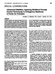
Several digital control techniques for dc-dc converters have been studied in this paper including current programming [8], estimative [9], predictive [10], dead-beat [1114], and digital [15, 16] methods. Although, different names have been adopted to present these methods in the literature, this study proves that they are all based on deadbeat control theory. All of these methods try to make the peak, average, or valley value of the inductor current follow a reference signal hereafter named iref. In most applications, iref or control signal is provided by the voltage compensator. Fig. 1.3 depicts the block diagram of a digital current-mode controller implemented using a DSP. Using samples of the inductor current and input and output voltages, the DSP tries to satisfy the control objective by finding the right value for the duty ratio. In current-mode control, the objective is to force the peak, average, or valley value of the inductor current to track reference current iref. The reference current itself is obtained from the voltage compensator.

10

iL

Vin

+ Vo -

Power Converter

A/D

d(t) iL[n] iref Current Controller reference

Voltage Controller

Vout[n] Vref[n]

current

DSP Figure 1.3. Block diagram of the digital current-mode controller

iL

ipeak[n] ipeak[n-1] iref[n-1]

iref[n]

iref[n-2]

iL[n-1]

iL[n-2]

iL[n]

d[n]Ts

d[n-1]Ts Ts (n-1)th period (n-2)Ts

t

Ts nth period (n-1)Ts

nTs

Figure 1.4. Actual and reference inductor current waveforms (in this figure average current-mode control is considered)

11 1.

General Equations of Buck Converter In this paper, without loss of generality, a buck converter is considered to

compare the dynamic response of different digital control methods. Typical inductor current waveform of a buck converter operating in continuous conduction mode is shown in Fig. 1.4. Input and output voltages are slowly varying signals and can be considered constant during one switching period. Therefore one car write Vo [n] ≈ Vo [n − 1] and Vin [n] ≈ Vin [n − 1]

(1)

Hence, for the sake of simplicity in notations in the following equations, input and output voltages are not shown as sampled signals even though they actually are. Provided that the input and output voltage samples, the inductance value, and the switching period are known, sampled inductor current iL[n] at time nTs, which is the end of the nth period, can be described as a function of previous sampled value iL[n-1] and applied duty ratio d[n]. Final value of the inductor current can be described as iL [n] = iL [n − 1] +

(Vin − Vo )d [n]Ts Vo (1 − d [n])Ts − L L

(2)

Solving (2) for d[n] would result d[n] =

L V (iL [n] − iL [n − 1]) + o VinTs Vin

(3)

Also, from (2), equations (4) and (5) can be derived. iL [n] = iL [n − 1] +

iL [n − 1] = iL [n − 2] +

Vin d [n]Ts VoTs − L L

(4)

Vin d [n − 1]Ts VoTs − L L

(5)

12 Where (5) is similar to (4) with one sample shift. Another way of obtaining equation (4) is using discrete state space averaging as mentioned in [16]. The average model of a buck converter is diL 1 d 1 = ( d ⋅ (Vin − Vo ) + (1 − d )(−Vo ) ) = Vin − Vo dt L L L

(6)

Writing the equivalent difference equation for (6) would result (4). By combining (4) and (5), we can extend (4) to another switching period to obtain iL [ n] = iL [ n − 2] +

Vin d [n − 1]Ts Vin d [n]Ts 2V0Ts + − . L L L

(7)

Solving (7) for the sample of duty ratio would result d[n] =

L 2V (iL [n] − iL [n − 2]) − d[n −1] + o VinTs Vin

(8)

Equation (9) can be derived based on (8) by one sample shift d[n −1] =

L 2V (iL[n −1] − iL[n − 3]) − d[n − 2] + o VinTs Vin

(9)

The following digital control techniques incorporate (3), (8), or (9) with their desired control objectives. 2.

Valley Current Control (method 1) This method is analog in nature [8]. However by changing the differential

equations describing the dynamic of the power converter to difference equations, a digital controller can be utilized to realize the control objective. A.

Control Objective In this control method, the required value for the duty cycle is calculated in the

ongoing period to make sure that

13 iL [n] = iref [n − 1]

(10)

In other words, final value of the inductor current is expected to follow the initial value of the reference sampled at the beginning of the switching cycle. One period of delay is intrinsic to the dead-beat control law. B.

Control Method Considering the control objective, by replacing iL[n] with iref[n-1] in (3), one

obtains

d [ n] =

V L (iref [n − 1] − iL [n − 1]) + o VinTs Vin

(11)

Therefore, in this control approach, inductor current iL, reference current iref, and voltages are sampled at the beginning of each switching period. Then (11) is used to calculate the required duty ratio so that final value of inductor current at the end of the switching cycle iL[n] will be equal with sampled reference current at the beginning of the switching cycle iref[n-1]. It is worth mentioning that this approach assumes that the digital signal processor (DSP) is fast enough to calculate the duty ratio and apply it immediately. A similar approach has been presented in [26]; however, it needs more time in calculations and therefore previous samples of input and output voltages are used. 3.

Average Current Control (method 2)

A.

Control Objective This method is introduced in [9]. The control objective is shown in equation (12).

That is the average value of inductor current in each switching cycle follows the reference current sampled at the beginning of the same period.

14

1 Ts

nTs ( n −1)Ts

iL (t )dt = iref [n − 1]

(12)

In Fig. 1.3, the average value of inductor current during the nth switching period can be calculated as 1 Ts

Ts [ n −1]Ts

iL (t ) dt =

1 ( Ts

d [ n ]Ts 0

(iL [n − 1] +

= i L [n − 1] +

Vin − Vo ⋅ t )dt + L

(1− d [ n ])Ts 0

(i L [ n − 1] +

Vin − Vo V d [n]Ts − o ⋅ t )dt ) L L

Vin d [n]Ts Vin d 2 [n]Ts Vo Ts − − L 2L 2L

(13)

Using (4), (13) can be further simplified to 1 Ts

nTs

( n −1)Ts

iL (t )dt = iL [n] +

VoTs Vin d 2 [n]Ts − 2L 2L

(14)

In order to satisfy the control objective, (14) has to be solved for d[n]. However, (14) in nonlinear and solution would need a long calculation time and includes truncation error. In order to simplify the solution of (14), duty ratio is replaced by its steady state value [10].

d [ n] ≈

Vo Vin

(15)

Applying (15) into (14) results

1 Ts

nTs ( n −1)Ts

iL (t )dt ≈ iL [n] +

TVo Vin − Vo ⋅ 2Vin L

(16)

B. Control Method This method assumes that the duty ratio calculated in every period can be used in the same period. To force the average value of the inductor current in the ongoing period to follow the reference sampled at the beginning of the same period and by combining (16), (12), and (3), one obtains

15

d [n] =

L T V V −V V (iref [n −1] − s o ⋅ in o − iL [n − 1]) + o . VinTs 2Vin L Vin

(17)

Therefore, using (17) to find the new value for the duty ratio will make sure that the control objective is satisfied. Valley current control, equation (11), and average current control, equation (17), can be compared using the following equation

d [ n] =

V L (iref [n − 1] − iL [n − 1] − K ) + o VinTs Vin

(18)

where the expression for K can be found in Table 1.1. Table 1.1. The Expression for K in Different Methods Method

K

Valley Control

0

Average Control

TsVo Vin − Vo ⋅ 2Vin L

4.

Delayed Valley Current Control (method 3)

A.

Control Objective This method is introduced in [10]. In this control method, the required value for

the duty cycle is calculated in the previous period to make sure that iL [n] = iref [n − 2]

(19)

In other words, the objective is to force the final (or valley) value of the inductor current in the ongoing period to follow the reference sampled at the beginning of the previous

16 period. This way, the digital controller will have more time for the required calculation; however, there is an extra period of delay introduced to the system. B.

Control Method This method assumes that the duty ratio of the ongoing period is calculated during

the previous switching period. By substituting the control objective in (8), one obtains iL [ n] = iL [ n − 2] +

Vin d [n − 1]Ts Vin d [n]Ts 2V0Ts + − L L L

(20)

If duty cycle d[n] is calculated based on (20) during the previous period and applied to the converter during the nth interval, then the inductor current will reach the reference current at the end of the nth interval and the dead-beat law is reached within two switching periods. It is worth mentioning that the digital controller has a longer time, compared with methods 1 and 2, to calculate the new value for the duty ratio. 5.

Delayed Peak Current Control

A.

Control Objective The control objective of this method is to force the peak value of the inductor

current during the ongoing period to follow the reference sampled at the beginning of the previous period. i peak [n] = iref [n − 2]

(21)

Where iref[n-2] is the reference current sampled at the beginning of the previous period. This control objective has less than two periods of time delay. B.

Control Method Equations (22) and (23) can be obtained from Fig. 1.3.

17

i peak [n] = i peak [n − 1] −

i peak [n − 1] = i peak [n − 2] −

Vo V −V (1 − d [n − 1])Ts + in o d [n]Ts L L

(22)

Vo V −V (1 − d [n − 2])Ts + in o d [n − 1]Ts L L

(23)

Substituting (23) into (22) and solving for d[n], one can find d [n ] =

L Vin Vo 2Vo (i peak [ n] − i peak [n − 2]) − d[ n − 1] − d [ n − 2] + (Vin − Vo )Ts Vin − Vo Vin − Vo Vin − Vo

(24)

Using control objective in (21), required duty ratio of the nth period can be described as d [ n] =

Vin Vo 2Vo L (iref [n − 2] − i peak [n − 2]) − d [n − 1] − d [n − 2] + (Vin − Vo )Ts Vin − Vo Vin − Vo Vin − Vo

(25)

Therefore, in this control approach, first peak value of the inductor current ipeak, reference current iref, and voltages are sampled in the previous period. Then (25) is used to calculate the required duty ratio so that the peak value of inductor current in the ongoing switching cycle ipeak[n] satisfies control objective (21). Similar to analog approaches, this method is unstable when the duty cycle is greater than 0.5 [11]. 6.

Delayed Average Current Control

A.

Control Objective The control objective of this method is shown in (26). That is the average current

value of nth period should follow the reference current sampled at the beginning of the previous period.

1 Ts

Ts [ n −1]Ts

iL (t ) = iref [n − 2]

(26)

18 B.

Control Method In [10], an approximation is made to solve (13) for d[n]. However, the solution is

unstable when the duty ratio is greater than 0.5. 7.

Prediction Current-Mode Control With Delay Compensation (method 4)

A.

Control Objective iL [n] = iref [n − 2]

(27)

This method is introduced in [11-14]. Its control objective is the same as method 3; however, the proposed approach is different. This control method has extended general equation (4) to four periods and the duty ratio is updated every two periods. The reference current is assumed as constant during these periods. B.

Control Method In [11-14], it is assumed the calculated duty ratio can be updated every other

period. This would provide more time for the required calculations. Equation (28) can be found in [11]

d [n] = d [n − 1] +

L (iref [n] − iL [n] d [ n−1] ) VinTs

(28)

Since reference current is assumed to be constant during a two period cycle, one can write iref [n] = iref [n − 2]

(29)

In this method, the current sampled at the end of nth period is assumed to be calculated from the current sampled at the end of the last two periods, which is shown in (30).

iL [ n ]

d [ n −1]

=2⋅iL [n − 1]

d [ n −1]

−iL [n − 2]

d [ n − 2]

(30)

19 If (29) and (30) are extended over three sampling periods and duty ratio is assumed to be upgraded every other period, equation (31) can be derived.

d [n] = d [n − 2] + = d [n − 2] +

(

1 L iref [n − 2] − i L [n − 1] d [ n −2 ] 2 VinTs

)

1 L (iref [n − 2] − 4iL [n − 2] + 3iL [n − 3]) 2 VinTs

(31)

Another way of deriving (31) is to use (9) and (1). By substituting (9) into (8), equation (32) can be obtained

d [n] =

L (iL [n] − iL [n − 2] − iL [n − 1] + iL [n − 3]) + d [n − 2] VinTs

(32)

From assumption (30), it can be observed that iL [n] =

1 ( iL [n +1] + iL [n −1]) 2

(33)

and iL [n − 1] = 2 ⋅ iL [n − 2] − iL [n − 3]

(34)

Substituting (33) and (34) into (31) and using the assumption of constant iref (35) can be obtained, which is the same as (31). d[ n] =

L (iref [n − 2] − 4iL [ n − 2] + 3iL [n − 3]) + d [n − 2] 2VinTs

(35)

Therefore, in this control approach, inductor current iL, reference current iref, and voltages are sampled in the previous three periods. Then (35) is used to calculate the required duty ratio so that final value of the inductor current at the end of the switching cycle iL[n] is equal with sampled reference current at the beginning of previous switching cycle iref[n-

20 2]. It is worth mentioning that the digital controller has at least two periods to calculate the new value for the duty ratio. 8.

Compensated Digital Current-Mode Control

A.

Control Objective This control method is introduced in [15] and [16]. The control objective can be

described in (36) iL [ n] = iref [ n − 1] + mc d [ n]Ts

(36)

Where, mc is a periodic compensating ramp. B.

Control Method By applying control objective (36) to general equation (3), one obtains d [ n] =

L V (iref [ n − 1] + mc d [n]Ts − iL [n − 1]) + o VinTs Vin

(37)

From (37), the final equation of this control method can be obtained as

d[n] =

V 1 L ( (iref [n −1] + mc d[n]Ts − iL [n − 1]) + o ) Lm Vin 1 − c VinTs Vin

(38)

If mc=0, then this control method is the same as valley current control (method 1). However, by applying periodic compensating ramp mc, this control method resolves stability issues that may occur in method 1. In order to make the system stable, there are some requirements for mc, which has been shown in Table 1.2.

21 Table 1.2. The Requirements for m Converter type buck boost buck-boost

9.

Requirement V mc > in L V mc > o L V −V mc > in o L

Summary of Different Digital Current-Mode Control Methods Table 1.3 compares the main characteristics of the most common digital current-

mode control approaches [28] including valley current control [9], average current control [10], delayed valley current control [11], and prediction current control with delay compensation [12-15]. The same notation is used in these methods. In most of these control methods, it is assumed that reference current iref is fairly constant.

22 Table 1.3. Conventional Digital Control Methods

Inherent Conventional

DSP processing

time delay

current control

Control objective

method

time limit (in

(in

Control method

switching

switching cycles)

cycles) Valley iL [n] = iref [n − 1]

L V (iref [ n − 1] − iL [ n − 1]) + o VinTs Vin

Less than one

L T V V −V V (iref [ n −1] − s o ⋅ in o − iL[ n −1]) + o VinTs 2Vin L Vin

Less than one

L 2V (iref [n − 2] − iL [n − 2]) − d[n − 1] + o VinTs Vin

One

L (iref [n − 2] − 4iL[n − 2] + 3iL [n − 3]) + d[n − 2] 2VinTs

One

d [ n] =

One

(method 1) Average

1 Ts

nTs

i (t ) dt = iref [ n − 1]

( n −1)Ts L

One

d [n ] =

(method 2) Delayed valley iL [n] = iref [n − 2]

Two

iL [n] = iref [n − 2]

Two

d [n] =

(method 3)

Prediction with delay compensation

d[n] =

(method 4)

As it can be observed from Fig. 1.4 and Table 1.3, in conventional valley and average digital current-mode control methods, samples of inductor current iL[n-1] and reference current iref[n-1] are provided at the beginning of the switching period. Using the control method, DSP should calculate the required duty ratio before the conduction time of the switch is over. The DSP processing time is less than one switching cycle in valley current control and average current control in Table 1.3, which is not long enough. The DSP processing time provided by conventional digital control methods is shown in Fig. 1.5. In order to solve this problem, an improved predictive digital control method is

23 introduced section IV. By using the proposed method, valley current control and average current control will have more time for the DSP to do the calculation. Delayed valley and prediction with delay compensation control methods have provided one switching cycle for the DSP processing time; however, they both have one period of extra time delay in their control objectives. samples are taken DSP calculations must be done by this time

iL

DSP processing time

t toff

toff

(n-2)Ts

(n-1)Ts

nTs

Figure 1.5. DSP processing time provided by conventional digital control methods

IV.

Improved Predictive Digital Control Using New Prediction

In order to provide more calculation time for the DSP, one would devise prediction methods for iL[n-1] and iref[n-1]. In that case, the DSP does not have to wait until the beginning of the switching cycle to sample iL[n-1] and iref[n-1]. These two signals will be predicted during the previous switching cycle right after the switch is turned off. The DSP processing time provided by proposed digital control method is shown in Fig. 1.6.

24

DSP calculations must be done by this time

iL Extra DSP processing time provided

t toff

toff (n-1)Ts

(n-2)Ts

nTs

Figure 1.6. DSP processing time provided by proposed digital control method 1.

Proposed Method to Predict iL[n-1] The final value of the inductor current in each period can be described as a

function of the initial value of the inductor current, positive and negative slopes, and the duration of the switch on and off times. Using Fig. 1.4, one could describe iL[n-1] as a function of previous samples that are already available in the DSP. In other words iL [n − 1] = iL [n − 2] +

(Vin − Vo )d [n − 1]Ts Vo (1 − d [n − 1])Ts − L L

(39)

Where, Ts is the switching period and L is the inductor value. Equation (39) can be simplified as iL [n − 1] = iL [n − 2] +

Vin d [n − 1]Ts VoTs − L L

(40)

25 It is worth mentioning that all the required samples on the right-hand side of (40) are already available in the DSP after the switch is turned off in the associated switching cycle. Equation (40) is used to predict iL[n-1]. 2.

Proposed Method to Predict iref[n-1] In order the predict iref[n-1], its previous samples are used. Using a slope

prediction approach, one can describe iref[n-1] as iref [ n − 1] = iref [ n − 2] + (iref [ n − 2] − iref [ n − 3]) = 2iref [ n − 2] − iref [ n − 3]

(41)

The relationship between predicted iref and real iref is shown in Fig. 1.7. iref[n-2]

iref[n-1]

iref[n-3] real iref

iref

Figure 1.7. The relationship between predicted iref and real iref For instance, by replacing the predicted values for iL[n-1] and iref[n-1] (equations (40) and (41)), the improved equation for the conventional valley control will be

d [ n] =

L V (2iref [n − 2] − iref [n − 3] − iL [n − 2]) − d [n − 1] + 2 o VinTs Vin

(42)

Table 1.4 depicts the control equation obtained by using the proposed method. Comparison between the control equation of Table 1.3 and 1.4 reveals that the proposed method does not impose any extra calculation time even though the related equations seem to be longer. The advantage here is that by using the proposed prediction method, more calculation time will be provided to the DSP. From the last columns of Table 1.3

26 and Table 1.4, it can be seen that the proposed methods offer more calculation time for DSP than conventional digital control methods. Table 1.4. Conventional Digital Control Methods Using Proposed Prediction

DSP

Proposed

processing

current Control objective

control

Control Equation

time limit (in switching

method

cycles) Predictive

L V (2iref [ n − 2] − iref [n − 3] − iL [n − 2]) − d [ n − 1] + 2 o VinTs Vin

One

L T V V −V V (2iref [ n − 2] − iref [n − 3] − iL [n − 2] − s o ⋅ in o ) − d [n − 1] + 2 o VinTs 2Vin L Vin

One

d [ n] =

iL [ n] = iref [ n − 1]

valley current control Predictive average current

1 Ts

nTs ( n −1)Ts

i L (t ) dt = iref [ n − 1]

d [ n] =

control

V.

Simulation Results

In order to study the dynamic performance of the proposed prediction method, a conventional digital average current control and its modified predictive counterpart are simulated and compared. The parameters of the buck converter are: Input voltage: Vin=6 V, Inductor value: L=108 uH, Capacitor value: C=92 uF, Switching frequency: fs=100 kHz, Load resistance: R=3 Ω, Reference current iref is 0.8 A with a low frequency peak to peak ripple of 0.4 A. Fig. 1.8 depicts the transient response inductor current for methods 1 through 4 if iref has a step change from 0.8 A to 1.2 A at t=0.003 s. All the currents are in Amps. The response of all methods is stable. It can be observed from Fig. 1.8 that the required time for methods 1 and 2 to track the reference is minimal. In method 1 valley value of the inductor current follows the reference whereas in method 2 average value of the inductor

27 current tracks the reference. In methods 3 and 4 there is one extra period of delay. This is due to compromise for a longer calculation time. Also, due to the predictions used in method 4, inductor current takes a loner time to reach the steady state.

iref

iL Valley current control (Method 1)

iL

Average current control (Method 2)

iL Delayed valley current control (Method 3)

iL

Prediction current control with delay compensation (Method 4)

iL Predictive valley current control

iL Predictive average current control

Figure 1.8. The transient response of methods 1 through 4, predictive valley current control, and predictive average current control to a step change in iref

28 Reference current, inductor current of conventional digital valley current-mode control, and inductor current of predictive digital valley current-mode control waveforms when reference current changes are shown in Fig. 1.9.

iref

Valley current control (method 1)

Predictive valley Current Control

Figure 1.9. Reference current, inductor current of conventional digital valley currentmode control, and inductor current of predictive digital valley current-mode control waveforms when reference current changes Waveforms of the inductor current and their reference according to the reference current change are shown in Fig. 1.10.

29

iref

Average current control (method 2)

Predictive average current control

Figure 1.10. Inductor current waveforms when reference current changes It can be seen from Fig. 1.10 that using the proposed prediction, the digital average current-mode control has the same performance as the conventional one. However, it has more time for the DSP to do the calculation. Therefore, the predictive average current-mode control can be used at higher frequency application. VI.

Conclusion

Several conventional digital current-mode control techniques were analyzed and compared in this paper. An improved prediction technique, which makes DSP realization of digital controllers easier, is also introduced in this paper. Conventional digital control methods reviewed in this paper do not perform very well when the switching frequency is high due to the fact that the DSP does not have enough time to perform all the required calculations. Using the proposed prediction method, the DSP will have a longer time for

30 processing purposes. The equations of several control methods modified by the improved prediction algorithm are listed in the paper. The simulation results show that the proposed prediction technique does not deteriorate the performance of the conventional digital control methods but at the same time offers more time for the DSP to do the calculations. It is also more practical than its conventional counterparts.

31 REFERENCES [1]

S. Cuk and R.D. Middlebrook, Advances in switched-mode power conversion, TESLA co., Pasadena, 1982, vol. 1, 1982.

[2]

R.D. Middlebrook and S. Cuk, “A general unified approach to modeling switchingconverter power stages,” in Proc. IEEE Power Electron., 1976, pp. 18-34.

[3]

R.W. Erickson, S. Cuk, and R.D. Middlebrook, “Large-signal modelling and analysis of switching regulators,” in Proc. IEEE Power Electron., 1982, pp. 240250.

[4]

C.W. Deisch, “Simple switching control method changes power converter into a current source,” in Proc. IEEE Power Electronics, 1978, pp. 135-147.

[5]

W. Tang, F.C. Lee, and R.B. Ridley, “Small-signal modeling of average currentmode control,” IEEE Trans. Power Electronics, vol. 8, no. 2, pp. 112-119, Apr. 1993.

[6]

L. Dixon, “Switching power supply control loop design,” in Proc. Unitrode Power Supply Design Sem., 1991, pp. 7.1-7.10.

[7]

C. Philip, “Modeling average current mode control [of power convertors],” in Proc. IEEE Applied Power Electronics Conference and Exposition, Feb. 2000, pp. 256262.

[8]

P. Shanker and J. M. S. Kim, “A new current programming technique using predictive control,” in Proc. IEEE International Telecommunications Energy Conference, Nov. 1994, pp. 428-434.

[9]

M. Ferdowsi, “An estimative current mode controller for dc-dc converters operating in continuous conduction mode,” in Proc. APEC, Mar. 2006, pp. 19-23.

[10] J. Chen, A. Prodic, R. W. Erickson, and D. Maksimovic, “Predictive digital current programmed control,” IEEE Trans. Power Electronics, vol. 18, no. 1, pp. 411-419, Jan. 2003.

[11] S. Bibian and J. Hua, “High performance predictive dead-beat digital controller for DC power supplies,” IEEE Trans. Power Electronics, vol. 17, no. 3, pp. 420-427, May 2002.

32 [12] S. Bibian and J. Hua, “Time delay compensation of digital control for DC switch mode power supplies using prediction techniques,” IEEE Trans. Power Electronics, vol. 15, no. 5, pp. 835-842, Sep. 2000. [13] S. Bibian and J. Hua, “A simple prediction technique for the compensation of digital control time delay in DC switch mode power supplies,” in Proc. IEEE Applied Power Electronics Conference and Exposition, Mar. 1999, pp. 994-1000.

[14] S. Bibian and J. Hua, “Digital control with improved performance for boost power factor correction circuits,” in Proc. IEEE Applied Power Electronics Conference and Exposition, Mar. 2001, pp. 137-143. [15] S. Chattopadhyay and S. Das, “A digital current-mode control technique for DC– DC converters,” IEEE Trans. Power Electronics, vol. 21, no. 6, pp. 1718-1726, Nov. 2006.

[16] C.C. Fang and E.H. Abed, “Sampled-data modeling and analysis of closed-loop PWM DC-DC converters,” in Proc. IEEE Int. Symp. Circuits and Systems, May 30Jun. 2, 1999, pp. 110-115. [17] G.C. Verghese, C.A. Bruzos, and K.N. Mahabir, “Averaged and sampled-data models for current mode control: a re-examination,” in Proc. IEEE Power Electronics Specialists Conference, 1989.

[18] F. Huliehel and S. Ben-Yaakov, “Low-frequency sampled-data models of switched mode DC-DC converters power electronics,” IEEE Trans. Power Electronics, vol. 6, no. 1, pp. 55-61, Jan. 1991. [19] G.C. Verghese, M.E. Elbuluk, and J.G. Kassakian, “A general approach to sampleddata modeling for power electronics circuit,” IEEE Trans. Power electronics systems, pp. 45-55, 1986.

[20] G. Francisco, C. Javier, P. Alberto, and M. Luis, “Large-signal modeling and simulation of switching DC-DC converters,” IEEE Trans. Power electronics, vol. 12, no. 3, May 1997. [21] A. Simon and O. Alejandro, Power-Switching Converters, 2nd edition. CRC press, 2005

33 [22] A. Brown and R.D. Middlebrook, “Sampled data modeling of switching regulators,” in Proc. IEEE Power Electronics Specialists Conference, 1981, pp. 349-369. [23] J. Weigold and M. Braun, “Robust predictive dead-beat controller for buck converters,” in Proc. IEEE Int. Power Electronics and Motion Control, Aug. 2006, pp. 951-956.

[24] O. Kukrer and H. Komurcugil, “Deadbeat control method for single-phase UPS inverters with compensation of computation delay,” in Proc. IEE Electric Power Applications, Jan. 1999, pp. 123-128. [25] K Wan, J. Liao, and M. Ferdowsi, “Control Methods in DC-DC Power Conversion – A Comparative Study,” in Proc. IEEE Power Electronics Specialists Conference, Jun. 2007, pp. 921-926.

[26] Z. Zhao and A. Prodic, “Continuous-Time Digital Controller for High-Frequency DC-DC Converters,” IEEE Trans. Power Electronics, vol. 23, no. 2, pp. 564-573, Mar. 2008. [27] S. Chae, B. Hyun, P. Agarwal, W. Kim, and B. Cho, “Digital Predictive FeedForward Controller for a DC–DC Converter in Plasma Display Panel,” in IEEE Trans. Power Electronics, vol. 23, no. 2, pp. 627-634, Mar. 2008. [28] S. Saggini, W. Stefanutti,, E. Tedeschi, and P. Mattavelli, “Digital Deadbeat Control Tuning for dc-dc Converters Using Error Correlation,” IEEE Trans. Power Electronics, vol. 22, pp. 1566-1570, July. 2007. [29] P. Mattavelli, L. Rossetto, and G. Spiazzi, “Small-signal analysis of DC-DC converters with sliding mode control,” IEEE Trans. Power Electronics, vol. 12, pp. 96-102, Jan. 1997. [30] L. Corradini, P. Mattavelli, and D. Maksimovic, “Robust Relay-Feedback Based Autotuning for DC-DC Converters,” in Proc. IEEE Power Electronics Specialists Conference, June. 2007, pp. 2196-2202. [31] L. Corradini, and P. Mattavelli, “Analysis of Multiple Sampling Technique for Digitally Controlled dc-dc Converters,” in Proc. IEEE Power Electronics Specialists Conference, June. 2006, pp. 1-6. [32] A. Parayandeh, and A. Prodic, “Programmable Analog-to-Digital Converter for Low-Power DC–DC SMPS,” IEEE Trans. Power Electronics, vol. 23 pp. 500-505, Jan. 2008.

34 [33] A. Prodic, and D. Maksimovic, “Mixed-signal simulation of digitally controlled switching converters,” in Proc. IEEE Workshop on Computers in Power Electronics, June. 2002, pp. 100-105. [34] Weaver, Wayne W, and Krein, Philip T, “Analysis and Applications of a CurrentSourced Buck Converter,” in Proc. IEEE Applied Power Electronics Conference, Mar. 2007, pp. 1664-1670. [35] M, Ilic, and D, Maksimovic, “Digital Average Current-Mode Controller for DC– DC Converters in Physical Vapor Deposition Applications,” IEEE Trans. Power Electronics, vol. 23, pp. 1428-1436, May. 2008. [36] D, Maksimovic, and R, Zane, “Small-Signal Discrete-Time Modeling of Digitally Controlled PWM Converters,” IEEE Trans. Power Electronics, vol. 22, pp. 25522556, Nov. 2007. [37] H, Peng, A. Prodic, E. Alarcon , and D. Maksimovic, “Modeling of Quantization Effects in Digitally Controlled DC–DC Converters,” IEEE Trans. Power Electronics, vol. 22, pp. 208-215, Jan. 2007. [38] J.T. Mossoba and P.T. Krein, “Small signal modeling of sensorless current mode controlled DC-DC converters,” in Proc. IEEE Computers in Power Electronics, Jun. 2002, pp. 23-28. [39] B. Miao, R. Zane, and D. Maksimovic, “Automated Digital Controller Design for Switching Converters,” in Proc. Power Electronics Specialists Conference, 2005, pp. 2729-2735.

35

Projected Cross Point – A New Average Current-Mode Control Approach K. Wan and M. Ferdowsi

Missouri University of Science and Technology Department of Electrical and Computer Engineering 1870 Miner Circle, Rolla, MO 65409, USA Tel: +1-573-341-4552, Fax: +1-573-341-6671 Email: [email protected] and [email protected]

Abstract-Projected cross point, a new current-mode control technique, is introduced and analyzed in this paper. While having an analog nature, the proposed method combines the advantages of both analog and digital control techniques. Unlike the conventional analog methods, it accurately controls the average value of the inductor current with no need to a current compensator or an external ramp. In addition, while resembling the deadbeat characteristics of digital controllers, projected cross point control does not suffer from computational time delay, limit cycling, and quantization and truncation errors.

Dynamic performance of the

proposed approach is compared with the existing control methods.

Analytical

analysis and simulation and experimental results show the superior accuracy and transient response of projected cross point control. Keywords-average current mode control; dc-dc converters; projected cross point control I.

Introduction

Analog approaches [1-9] including voltage- and current-mode control have conventionally been used to provide line and load regulation in dc-dc power converters.

36 They are very popular due to their simplicity, high bandwidth, and low implementation cost. The main disadvantage of analog current-mode controllers is the need for external ramp compensation. As a result of this, the inductor current does not accurately track the reference current; hence, in most of the operating situations, the current control loop is over-compensated and therefore slow. Digital controllers have had a substantial development over the past few years [10-36]. Although digital control schemes have several advantages compared to analog approaches, they have several disadvantages including high cost, computational time delay, limit cycling, and quantization and truncation errors. Projected cross point control (PCPC), a new average current-mode control technique, is introduced in this paper. PCPC is analog in nature; however, it resembles the deadbeat characteristic of digital approaches. PCPC does not need a current compensator and controls the true average value of the inductor current with no subharmonic oscillations. It has a very fast dynamic response and is not sensitive to the output voltage noise. PCPC avoids the disadvantages of digital controllers. PCPC first projects the equation of the inductor current in the negative slope area; then, it locates the cross point of the positive slope inductor current and the projected line to find the accurate value of the duty ratio. PCPC method can be realized by analog parts and there is no need for a digital signal processor. In Section II, advantages and disadvantages of conventional current-mode control is presented. Digital control of dc-dc converters is briefly reviewed in Section III. Principles of operation and implementation of PCPC are provided in Section IV. Comparison among the dynamic performance of the conventional current-mode

37 controllers, digital control method, and PCPC approach are discussed in Section V. In Section VI, the PCPC method is implemented and experimentally verified using a boost converter. Finally, Section VII draws the conclusions and presents an overall evaluation of the newly proposed control method. II. 1.

Analog Control Techniques

Voltage-Mode Control of dc-dc Converters Conventional analog control approaches for dc-dc converters used in industry

include voltage-mode and current-mode control. Voltage-mode control is a single-loop controller (see Fig. 2.1). It uses measured output and reference voltage to generate the control voltage. Then the control voltage is used to determine the switching duty ratio by comparison with a fixed frequency sawtooth waveform. This switching duty ratio is used to adjust the average voltage across the inductor and therefore the inductor current. This will eventually bring the output voltage to its reference value. Voltage-mode control of dc-dc converters has several disadvantages including 1) poor reliability of the main switch, 2) degraded reliability, stability, or performance when several parallel converters supply one load, 3) complex and often inefficient methods of keeping the main transformer of a push-pull converter operating in the center of its linear region, and 4) a slow system response time which may be several tens of switching cycles.

38

Power Converter

Vin

Vc d

Compensator

+ -

Vo Ve

+

Vref

Figure 2.1. Block diagram of a voltage-mode controller 2.

Current-Mode Control of dc-dc Converters Current-mode control is a dual loop control method, including current and voltage

control loops. In this method, the error signal between output voltage vo and reference voltage vref is used to generate reference current iref. Then, this reference current is compared with sensed inductor current iL to control the duty cycle, as shown in Fig. 2.2. Through this method, the inductor current will track reference current iref and the output voltage will become equal to reference voltage vref. There are three basic types of currentmode control techniques which are peak, valley, and average current-mode control methods. Compared with voltage mode control, current-mode control has many advantages and a few disadvantages which will briefly be discussed below.

39

Power Converter

Vin

Vo

d iL(t) S

Clock

Q R

+ -

Compensator

Ve

- Vref +

iref(t) Figure 2.2. Block diagram of a peak current-mode controller A.

Advantages of Current-mode Control A converter with a current-mode controller has additional good properties which

many other converters lack. a. Improved transient response. The current-mode control converter is a first order system. It is much easier to design a feedback circuit and the overall transient response is greatly improved. b. Output immunity to the input noise The output of the constant current converter is nearly independent of the input. It puts a fixed current into the load so input transients do not have to be corrected by external feedback. c. Suitable in paralleled converters If it is used in paralleled converters, there is only one external feedback circuit to regulate the voltage. The paralleled converters received the same control voltage, so there is equal load sharing. d. Self-protection against overload

40 The current-mode control converter needs no short circuit protection because it is a current source. The control voltage is internally limited, so even if the external control voltage goes to some high values, the current output just goes to its maximum. Although the converter behaves as a current source, it does not suffer the disadvantage of the needing open circuit protection. The maximum output voltage is limited by the transformer turns ratio, the same as a conventional voltage converter. e. Over-current protection for the main switches The current threshold is internally limited to a maximum value. So the maximum switch current is automatically limited. This feature improves reliability by protecting the switches during startup, overloads, and other potentially damaging transients. f. Anti-saturation which keeps the main transformer core in the center of its B-H curve. The current threshold control circuit automatically keeps the core in the center of the B-H curve because the current in each switch is shut off at the same level. Any magnetizing current unbalance automatically causes the switch timing to cancel the unbalance and there is near zero dc voltage applied to the transformer primary. B.

Disadvantages of Current-Mode Control It will become unstable when the duty ratio exceeds 0.5 in peak current-mode

control. This effect is explained in Fig. 2.3. In this figure, the solid line is the inductor current waveform of the converter in steady state, while the dashed line shows the waveform of the perturbed inductor current.

41

reference current iref -m2

∆I 0

m1

inductor current iL

∆I1

(1-d)Ts

dTs

t

Figure 2.3. Propagation of a perturbation in current-mode control: instability occurs when d is greater than 0.5 In steady state, the inductor current has a rising slop m1 and a falling slope –m2. If there is a perturbation of I0 in the inductor current relative to the steady state at the beginning of a period, after n periods, this perturbation will become m ∆I n = − 2 m1

n

∆I 0 = −

d 1− d

n

∆I 0

(1)

where d is the duty ratio. Equation (1) shows that the error will be enlarged after several cycles and the system will become unstable when the duty ratio is greater than 0.5. Adding an external ramp can solve this problem. A cyclic falling slope –m is added to the reference current in Fig. 2.4.

42

reference current iref -m

external ramp

inductor current iL -m2

∆I 0

m1

∆I1 (1-d)Ts

dTs

t

Figure 2.4. Propagation of a perturbation in the programmed current: in the presence of a suitable ramp, stability can be maintained for all d From Fig. 2.4, by using the external ramp –m, the perturbation I0 will become ∆I n = −

m2 − m m1 + m

n

∆I 0

(2)

after n cycles. It can be seen from (2), the perturbation will die out after several cycles if the external ramp -m is selected appropriately, even if the duty ratio is greater than 0.5. In particular, m is chosen to be equal to m2. Thus, the perturbation of the inductor current will disappear in one cycle. The system will be stable and simultaneously provide the fastest possible transient response of the current mode control. In average current-mode control, a low-pass filter is used after current sensor to get the average value of the inductor current. This filter causes some time delay in the current loop which deteriorates the dynamic response. III.

Digital Current-Mode Control

Different kinds of digital controllers have been introduced recently [10-25]. Fig. 2.5 depicts the block diagram of a digital current-mode controller implemented using a

43 DSP. In digital current-mode control, the sampled inductor current and input and output voltages are used to compute the duty ratio in the next switching cycle so that the error between the reference current and the target control variable is reduced to zero. In digital current-mode control, the objective is to force the peak, average, or valley value of the inductor current to follow reference current iref. In most applications, the reference current itself is obtained from the digital voltage compensator.

iL Power Converter

Vin

+ Vo A/D

d(t) iL[n] iref Current Controller reference

Voltage Controller

Vout[n] Vref[n]

current

DSP Figure 2.5. Block diagram of the digital current-mode controller 1.

Advantages of Digital Current-Mode Control Compared with analog circuit, digital control system offers a numbers of

advantages. Digital control has high flexibility. In digital control, different control algorithms can be easily implemented by software in the same hardware control system. It can be easily and fast changed according to the design requirement. Communication, protection,

44 prevention and monitoring circuits could be easily built in the digital control system. Fewer components are used in digital control compared with analog circuit. Hence, digital control system has better reliability than analog circuits. It is much easier to implement the advanced control techniques into digital control system. As a result, the system dynamic performance could be significantly improved. 2.

Disadvantages of Digital Current-Mode Control One of the main drawbacks of digital control is the limited bandwidth due to the

inherent time delay required for A/D conversion, computation, and PWM generation. In switch mode power supplies, this delay is usually equal to one sampling period. Such time delay degrades the control loop performance, resulting in slower response and less rejection to dc bus ripples and load disturbances. Also, the signal amplitude quantizers such as A/D converters used in digital control cause the problems of limit cycle. It is hard to predict the amplitude and frequency of the limit cycle. It causes undesirable and unpredicted output voltage variations in the steady-state. It also brings difficulties in the analysis and compensation of noise and electro-magnetic interference in power electronic converters. DSP should be used to realize digital current-mode control. So the high cost is also a drawback of digital control methods. IV.

Projected Cross Point Control Approach

In this paper, without loss of generality, a buck converter is used to introduce the principles of operation of projected cross point control (PCPC) method. Typical waveform of the inductor current is shown in Fig. 2.6. In this figure, iref indicates the reference current, which is the output signal of the voltage compensator. Without loss of

45 generality and for the ease of demonstration in Fig. 2.6, reference current iref is drawn as a straight line. The desired inductor current in the steady-state is sketched in dashed lines and associated labels are identified by an ss (steady state) subscript. It is worth mentioning that the initial and final values of the inductor current in the steady-state operation are identical and the average value of the inductor current follows the current reference. In Fig. 2.6, perturbed inductor current is sketched in solid lines. The control objective is to make sure that the final value of the inductor current returns to its steady state value no matter what the initial value of the inductor current is. In other words iL (t = nTs ) = i fin, ss = iref −

∆iL 2

(3)

where, ifin,ss is the final value of the inductor current in the steady state operation and iL is the steady-state peak-to-peak ripple of the inductor current. It is obvious that if the control objective is satisfied, in the next switching cycle, average value of the inductor current will be identical with the reference current and hence PCPC is an average currentmode control approach.

a iL i−

I ini

∆ iL 2

iref

I fin = I fin ,ss

I ini ,ss (n-1)Ts

ton

ton, ss

nTs

Figure 2.6. Typical current waveform of a buck converter

∆ iL 2

46 In order to satisfy the control objective, the proposed controller needs to find the cross point of lines iL and i - (the inductor current in the negative slope area) which is indicated as point ‘a’ in Fig. 2.6. The equation for i – is i − = i ref −

∆i L vo v + Ts − o t 2 L L

(4)

In order to find ton, the cross point of iL and (4) will have to be identified; therefore, i L (t = t on ) = i − (t = t on ) .

i L (t = t on ) = i ref −

(5)

. ∆i L v o v + Ts − o t on 2 L L

(6)

Equation (6) can be simplified as L(iL (t = ton ) − iref (t = ton ) + ∆iL / 2) = voTs − voton

(7)

PCPC solves (7) for ton in real time as shown in the block diagram in Fig. 2.7. Different expressions in (7) that are labeled (a) through (e) are found as follows. (a) Inductor current iL is measured. (b) Reference current iref is measured. (c) steady-state peak-to-peak ripple of the inductor current.

iL is the

iL/2 is found based on the

previous measured values of iL and iref, as shown in Fig. 2.8.

imax is defined as the

difference between the maximum value of iL and iref sampled at the turn-off time of the switch, which is generated by the reset input of the SR flip-flop. imin is defined as the difference between the minimum value of iL and iref sampled at the turn-on time of the switch, which is generated by the clock signal. Average values of

imax and

imin,

measured in each switching cycle, are then found by a simple analog circuitry. iL/2 is then found using a low pass filter (LPF). An LPF is used to make sure that transients and

47 tracking errors have no effect on the accurate measurement of iL/2. The transfer function of LPF used in this work is (1+80*10-6S)-1. (d) Output voltage is relatively constant; therefore, voTs can be found by integrating the output voltage over the previous switching cycle. (e) voton cab be found by integrating the output voltage during the on-time of the switch. PCPC method can be compared with its digital counterparts. The equation of iL is shown in (8), iL = I ini +

Vin − Vo t L

(8)

From (4), (5), and (8), one obtains Vin ∆i VT t on = iref − L + o s − I ini L 2 L

(9)

The following are some standard notions in digital applications, I ini = i L [ n − 1] , i ref = i ref [n − 1] , t on = d [ n]Ts

(10)

Substituting (10) into (8), one obtains Vin ∆i V T d [n]Ts = iref [ n − 1] − iL [n − 1] − L + o s L 2 L

(11)

which can be expressed as, d [n ] =

L T V V −V V (iref [ n − 1] − iL [ n − 1] − s o ⋅ in o ) + o VinTs 2Vin L Vin

(12)

Equation (12) is the same equation of average digital current-mode control method introduced in [10] and [11].

48 L (c) ∆iL / 2

(a) iL(t)

Clock + + -

+

-

reset

Power Converter

Vin

Ts

Vo

(d)

0

(e)

0

t on

d

S/H +

Voton

S/H

S Q R

-

reset

- Ve

Vref +

V oT s

Voltage loop compensator (b) iref(t)

Figure 2.7. Block diagram of the PCPC approach

iL

S/H

S Q R iref iL

imax + -

S/H S/H

iref imin + -

clock

iref

+ -

S/H

iref

0.5

iL

∆imax + ∆imin 2

imax

LPF

∆ iL 2

∆imax

iref imin ∆imin

Figure 2.8. Block diagram of the steady-state peak-to-peak ripple finder V.

Simulation Results

In order to observe the performance of the new proposed method, a peak current mode controller with external ramp is used. A buck converter with the following parameters is used as the power stage.

49 Reference voltage Vref = 2 V, Inductor value L = 20 uH, Capacitor value C = 330 uF, Switching frequency fs = 100 kHz, Input voltage Vin abruptly changes from 3 V to 6 V at 0.003 s, and Load resistance R abruptly changes from 2 Ω to 3 Ω at 0.02s. The voltage loop compensator of these control methods is the same, which is

27447 1/(6.0518*103 ) s + 1 s 1/(1.3076*105 ) s + 1

(13)

Figure. 2.9 depicts the tracking accuracy of PCPC scheme. In this simulation, voltage loop is open and reference current iref is subjected to positive and negative step changes and slopes. As it can be observed, the inductor current can precisely track its reference with no time delay. PCPC truly and accurately controls the average value of the inductor current. Furthermore, there is no sign of sub-harmonic oscillations. Having the voltage loop closed, waveforms of the output voltage and the inductor current and its reference when there is a step change in input voltage Vin are shown in Figs. 2.10 and 2.11, respectively. The results show that the proposed current control method has a superior transient performance for line regulation. Waveforms of the output voltage and the inductor current and its reference when there is a step change in the load resistance are shown in Figs. 2.12 and 2.13, respectively. The performance of peak current mode control with an external ramp that is smaller or larger than optimal ramp is shown in Fig. 2.14. It is shown in Fig. 2.14 that the peak current mode control with a smaller external ramp performs better in transients but worse in steady state. The peak current mode control with a larger external ramp performs better in steady state but worse in transients. Fig. 2.15 shows the output voltage waveforms of PCPC method and digital control

50 method when reference current changes from 0.8A to 1.2A at 0.002s. It can be seen from Fig. 2.15 that the PCPC method matches the performance of digital method. But in the digital control method in Fig. 2.15, it assumed that the DSP is fast enough to calculate the next duty cycle before the switch is turned off.

Figure 2.9. The inductor current waveform using PCPC approach

51

PCPC approach

peak current-mode control with optimal ramp

peak current-mode control with larger ramp

peak current-mode control with smaller ramp

Figure 2.10. Inductor current and its reference waveforms when Vin changes from 3 V to 6 V at 0.003 s PCPC approach

optimal ramp

larger ramp

smaller ramp

Figure 2.11. Output voltage waveforms when load changes from 2 Ω to 3 Ω at 0.005 s

52

PCPC approach

peak current-mode control with optimal ramp

peak current-mode control with larger ramp

peak current-mode control with smaller ramp

Figure 2.12. Inductor current and its reference waveforms when load changes from 2 Ω to 3 Ω at 0.005 s

PCPC approach

optimal ramp

larger ramp

smaller ramp

Figure 2.13. Transients in the output voltage when input voltage Vin changes from 3 V to 6 V at 0.003 s

53 PCPC approach

optimal ramp

larger ramp

smaller ramp

Figure 2.14. Steady state in the output voltage when input voltage Vin changes from 3 V to 6 V at 0.003 s

PCPC method

Average digital control method

Figure 2.15. Output voltage of PCPC method and digital control method when iref current changes from 0.8A to 1.2A at 0.002s

54 VI.

Experimental Results

A boost converter is designed and tested to validate the idea of PCPC method. The parameters of this converter are shown in Table 2.1. Table 2.1. Converter Main Parameter and Specifications Nominal Values: Output voltage Dc bus voltage Switching period Output filter: Inductor Capacitor Load:

Vo 21V Vin 14V Ts 10µs L 125uH C 820uF R 60

Figures. 2.16 and 17 show the inductor current when iref changes from 1.52A to 1.42A and from 1.47A to 1.56A respectively. It can be seen from Fig. 2.16 and Fig. 2.17 that inductor current tracks the reference current very well. With the voltage compensation loop closed, inductor current waveforms according to the drop and rise of input voltage are shown in Fig. 2.18 and Fig. 2.19 and the output voltage waveforms according to the drop and rise of input voltage are shown in Fig. 2.20 and Fig. 2.21. It can be seen from Fig. 2.18, Fig. 2.19, Fig. 2.20, and Fig. 2.21 that PCPC method has an excellent performance in line regulation.

55

inductor current reference current iref

Figure 2.16. Inductor current waveform when iref changes from 1.52A to 1.42A

reference current iref inductor current

Figure 2.17. Inductor current waveform when iref changes from 1.47A to 1.56A

56

input voltage

inductor current

Figure 2.18. Inductor current waveform when input voltage drops from 14V to 10.5V

input voltage

inductor current

Figure 2.19. Inductor current waveform when input voltage rises from 10.5V to 14V

57

output voltage

input voltage

Figure 2.20. Output voltage waveform when input voltage drops from 14V to 10.5V

output voltage

input voltage

Figure 2.21. Output voltage waveform when input voltage rises from 10.5V to 14V

58 VII.

Conclusion

Projected cross point control (PCPC), a new average current-mode control, method is presented in this paper. In each switching cycle, it finds the duty ratio based on the point where the real inductor current and the steady state negative slope inductor current cross each other. The proposed method is analog based and simple. It is cheap to implement and has a very fast dynamic response. Compared with digital approaches, the proposed control method does not suffer from computational time delay, limit cycle, and truncation problems. It can match the transient performance of digital control methods. Compared with conventional analog approaches, the presented control scheme is stable for all values of the duty ratio; hence, it does not need any external ramp compensation. Furthermore, PCPC does not need any current compensation circuit. In addition, it accurately controls the true average value of the inductor current. Simulation results prove its superior transient performance. Experiment results also show that PCPC method has good performance in load and line regulation.

59 REFERENCES

[1]

C.W. Deisch, “Simple switching control method changes power converter into a current source,” in Proc. IEEE Power Electronics Specialists, 1978, pp. 135-147.

[2]

S. Cuk and R.D. Middlebrook, Advances in switched-mode power conversion, TESLA co., Pasadena, 1982, vol. 1, 1982.

[3]

R.D. Middlebrook and S. Cuk, “A general unified approach to modeling switchingconverter power stages,” in Proc. IEEE Power Electron., 1976, pp. 18-34.

[4]

R.W. Erickson, S. Cuk, and R.D. Middlebrook, “Large-signal modelling and analysis of switching regulators,” in Proc. IEEE Power Electron., 1982, pp. 240250.

[5]

W. Tang, F.C. Lee, and R.B. Ridley, “Small-signal modeling of average currentmode control,” IEEE Trans. Power Electronics, vol. 8, no. 2, pp. 112-119, Apr. 1993.

[6]

L. Dixon, “Switching power supply control loop design,” in Proc. Unitrode Power Supply Design Sem., 1991, pp. 7.1-7.10.

[7]

C. Philip, “Modeling average current mode control [of power convertors],” in Proc. IEEE Applied Power Electronics Conference and Exposition, Feb. 2000, pp. 256262.

[8]

A. Simon and O. Alejandro, Power-Switching Converters, 2nd edition. CRC press, 2005

[9]

A. Brown and R.D. Middlebrook, “Sampled data modeling of switching regulators,” in Proc. IEEE Power Electronics Specialists Conference, 1981, pp. 349-369.

[10] M. Ferdowsi, “An estimative current mode controller for dc-dc converters operating in continuous conduction mode,” in Proc. APEC, Mar. 2006, pp. 19-23. [11] K. Wan, J. Liao, and M. Ferdowsi, “Control methods in dc-dc power conversion – a comparative study,” in Proc. IEEE Power Electronics Specialists Conference, Jun. 2007, pp. 921-926 [12] P. Shanker and J. M. S. Kim, “A new current programming technique using predictive control,” in Proc. IEEE International Telecommunications Energy Conference, Nov. 1994, pp. 428-434.

60 [13] J. Chen, A. Prodic, R. W. Erickson, and D. Maksimovic, “Predictive digital current programmed control,” IEEE Trans. Power Electronics, vol. 18, no. 1, pp. 411-419, Jan. 2003. [14] S. Bibian and J. Hua, “High performance predictive dead-beat digital controller for DC power supplies,” IEEE Trans. Power Electronics, vol. 17, no. 3, pp. 420-427, May 2002. [15] S. Bibian and J. Hua, “Time delay compensation of digital control for DC switch mode power supplies using prediction techniques,” IEEE Trans. Power Electronics, vol. 15, no. 5, pp. 835-842, Sep. 2000. [16] S. Bibian and J. Hua, “A simple prediction technique for the compensation of digital control time delay in DC switch mode power supplies,” in Proc. IEEE Applied Power Electronics Conference and Exposition, Mar. 1999, pp. 994-1000.

[17] S. Bibian and J. Hua, “Digital control with improved performance for boost power factor correction circuits,” in Proc. IEEE Applied Power Electronics Conference and Exposition, Mar. 2001, pp. 137-143. [18] S. Chattopadhyay and S. Das, “A digital current-mode control technique for DC– DC converters,” IEEE Trans. Power Electronics, vol. 21, no. 6, pp. 1718-1726, Nov. 2006. [19] C. C. Fang and E. H. Abed, “Sampled-data modeling and analysis of the power stage of PWM dc-dc converters,” Technical Research Report, 1999. [20] G.C. Verghese, C.A. Bruzos, and K.N. Mahabir, “Averaged and sampled-data models for current mode control: a re-examination,” in Proc. IEEE Power Electronics Specialists Conference, 1989. [21] F. Huliehel and S. Ben-Yaakov, “Low-frequency sampled-data models of switched mode DC-DC converters power electronics,” IEEE Trans. Power Electronics, vol. 6, no. 1, pp. 55-61, Jan. 1991. [22] G.C. Verghese, M.E. Elbuluk, and J.G. Kassakian, “A general approach to sampleddata modeling for power electronics circuit,” IEEE Trans. Power electronics systems, pp. 45-55, 1986. [23] G. Francisco, C. Javier, P. Alberto, and M. Luis, “Large-signal modeling and simulation of switching DC-DC converters,” IEEE Trans. Power electronics, vol. 12, no. 3, May 1997.

61 [24] J. Weigold and M. Braun, “Robust predictive dead-beat controller for buck converters,” in Proc. IEEE Int. Power Electronics and Motion Control, Aug. 2006, pp. 951-956. [25] O. Kukrer and H. Komurcugil, “Deadbeat control method for single-phase UPS inverters with compensation of computation delay,” in Proc. IEE Electric Power Applications, Jan. 1999, pp. 123-128. [26] P. Mattavelli, L. Rossetto, and G. Spiazzi, “Small-signal analysis of DC-DC converters with sliding mode control,” IEEE Trans. Power Electronics, vol. 12, pp. 96-102, Jan. 1997 [27] L. Corradini, P. Mattavelli, and D. Maksimovic, “Robust Relay-Feedback Based Autotuning for DC-DC Converters,” in Proc. IEEE Power Electronics Specialists Conference, June. 2007, pp. 2196-2202. [28] L. Corradini, and P. Mattavelli, “Analysis of Multiple Sampling Technique for Digitally Controlled dc-dc Converters,” in Proc. IEEE Power Electronics Specialists Conference, June. 2006, pp. 1-6. [29] A. Parayandeh, and A. Prodic, “Programmable Analog-to-Digital Converter for Low-Power DC–DC SMPS,” IEEE Trans. Power Electronics, vol. 23 pp. 500-505, Jan. 2008. [30] A. Prodic, and D. Maksimovic, “Mixed-signal simulation of digitally controlled switching converters,” in Proc. IEEE Workshop on Computers in Power Electronics, June. 2002, pp. 100-105. [31] Weaver, Wayne W, and Krein, Philip T, “Analysis and Applications of a CurrentSourced Buck Converter,” in Proc. IEEE Applied Power Electronics Conference, Mar. 2007, pp. 1664-1670. [32] M, Ilic, and D, Maksimovic, “Digital Average Current-Mode Controller for DC– DC Converters in Physical Vapor Deposition Applications,” IEEE Trans. Power Electronics, vol. 23, pp. 1428-1436, May. 2008. [33] D, Maksimovic, and R, Zane, “Small-Signal Discrete-Time Modeling of Digitally Controlled PWM Converters,” IEEE Trans. Power Electronics, vol. 22, pp. 25522556, Nov. 2007. [34] H, Peng, A. Prodic, E. Alarcon , and D. Maksimovic, “Modeling of Quantization Effects in Digitally Controlled DC–DC Converters,” IEEE Trans. Power Electronics, vol. 22, pp. 208-215, Jan. 2007.

62 [35] J.T. Mossoba and P.T. Krein, “Small signal modeling of sensorless current mode controlled DC-DC converters,” in Proc. IEEE Computers in Power Electronics, Jun. 2002, pp. 23-28. [36] B. Miao, R. Zane, and D. Maksimovic, “Automated Digital Controller Design for Switching Converters,” in Proc. Power Electronics Specialists Conference, 2005, pp. 2729-2735.

63

Self-Tuned Projected Cross Point - An Improved Current-Mode Control Technique K. Wan and M. Ferdowsi

Missouri University of Science and Technology Department of Electrical and Computer Engineering 1870 Miner Circle, Rolla, MO 65409, USA Tel: 001-573-341-4552, Fax: 001-573-341-6671 Email: [email protected] and [email protected]

Abstract — Self-tuned projected cross point control for power supplies and power electronic converters is presented in this paper. Projected cross point control (PCPC) combines the advantages of both analog and digital current-mode control techniques. Despite several advantages, accuracy of PCPC method depends on the power stage inductor value. However, ferromagnetic characteristic of the inductor makes the inductor measurement inaccurate. Furthermore, the inductor value is subject to change due to temperature variations or other environmental effects. To overcome the dependence of PCPC method on the inductor value, self-tuned PCPC approach introduced in this paper. Unlike conventional PCPC scheme, self-tuned PCPC method has excellent robustness against the variation of inductor value. It self-adjusts the inductor value, which is used in the control stage, according to the error between the average inductor current and reference current. Hence, the average inductor current accurately follows its reference regardless of aging and temperature effects on the power stage inductor. Furthermore, addition of selftuning mechanism does not interfere with the performance of conventional PCPC

64

method. Analytical analysis, simulation and experimental results show the superior accuracy and transient response of self-tuned projected cross point control technique. Keywords-average current mode control; dc-dc converters; projected cross point control I.

Introduction

Projected cross point control (PCPC) technique has been introduced in [1]. It enjoys the advantages of both analog and digital current-mode control techniques. Unlike the conventional analog methods [2-15], it accurately controls the average value of the inductor current with no need of a current compensator or an external ramp. In addition, while resembling the deadbeat characteristics of digital current-mode controllers [16-39], PCPC method does not suffer from computational time delay, limit cycling, and quantization and truncation errors. Despite its excellent advantage, accuracy of PCPC method depends on the power stage inductor value. Inductor value has to be measured and preprogrammed in the controller. However the following reasons make it is difficult to get the accurate inductor values during the dc-dc converter design. 1). Measurement of inductor value. The measurement of inductor values is not accurate enough. All the inductor values offered by the manufacturer are measured under normal conditions. Most measurement devices measure the inductor values under low magnetic field intensity. But the saturate degrees of the core of inductor are different when the environment changes. So the actual inductor values will be different with the measured ones. 2). Nonlinear characteristic of inductor. Inductor is a nonlinear component. Its value will be changed according to the

65 saturation degree of the core and the current passing through it. 3). Temperature. When the temperature changer, the inductor values will also be changed. 4). Effect of other components. Other components used in dc-dc converters such as capacitor have equivalent serial inductance, which will work together with the inductor. The equivalent serial inductance will also change the actual inductor value used in dc-dc converters. Furthermore, power stage inductor value is subject to change due to temperature, aging, and the dc current passing through it. Therefore, PCPC approach will not be accurate enough if one fails to find or estimate the exact value for the inductor. Otherwise, there will be an offset between the inductor current and its reference. In other words, control objective will not be satisfied anymore. An improved PCPC method, named self-tuned PCPC technique, is introduced in this paper. Self-tuned PCPC method uses the error between the inductor current and its reference to adjust the inductor value used in the controller. As a result, the control objective is satisfied and improved. The controller is robust against variations of the power stage inductor value. Self-tuning does not interfere with line and load regulations; hence, self-tuned PCPC method has identical regulation dynamic as the conventional one. In Section II, principles of operation and implementation of PCPC scheme are provided. Self-tuned PCPC method is discussed in detail in Section III. Simulation results are presented in Section IV. A boost converter is built and tested to verify the validity of improved PCPC method in Section V. Finally, Section IV draws the conclusions and presents an overall evaluation of self-tuned PCPC approach.

66 II. 1.

Projected Cross Point Control Approach

Introduction of Projected Cross Point Control Method PCPC method has been introduced in [1]. In this paper, without loss of generality,

a buck converter is used to introduce the principles of operation of projected cross point control (PCPC) method. A typical waveform of the inductor current is shown in Fig. 3.1. In this figure, iref indicates the reference current, which is the output signal of the voltage compensator. Without loss of generality and for the ease of demonstration in Fig. 3.1, reference current iref is drawn as a straight line. Desired inductor current in steady-state operation is sketched in dashed lines. Associated labels are identified by an ss (steadystate) subscript. It is worth mentioning that, in average current-mode control and under steady-state conditions, initial and final values of the inductor current are identical and average value of the inductor current follows the reference current. In Fig. 3.1, perturbed inductor current is sketched in solid lines. Considering average current-mode control, the control objective is to make sure that final value of the inductor current returns to its steady-state value no matter what the initial value of the inductor current is. In other words iL (t = nTs ) = I fin , ss = iref −

∆iL 2

(1)

Where, Ifin,ss is the final value of the inductor current in steady state operation and iL is the steady-state peak-to-peak ripple of the inductor current. It is obvious that if the control objective is satisfied, in the next switching cycle, average value of the inductor current will be identical with the reference; therefore, PCPC is an average current-mode control approach.

67

a iL i-

Iini

∆ iL 2

iref Ifin = Ifin,ss

Iini,ss ton

(n-1)Ts

ton,ss

∆ iL 2

nTs

Figure 3.1. Typical inductor current waveform of a buck converter In order to satisfy the control objective, PCPC method needs to find the cross point of lines iL and i - (the inductor current in the negative slope area), which is indicated as point ‘a’ in Fig. 3.1. The equation for i – is i − = iref −

∆iL vo v + Ts − o t 2 L L

(2)

In order to find ton, the cross point of iL and i – will have to be identified; therefore, i L = I ini +

vin − vo t L

(3)

By combining (3) and (4), one obtains iL (t = ton ) = iref −

∆iL vo v + Ts − o ton 2 L L

(5)

Equation (5) can be simplified as Lreal * [iL (t = ton ) − iref (t = ton ) + ∆iL / 2] = voTs − voton (a)

(b)

(c)

(d)

(6) (e)

PCPC scheme solves (6) for ton in real time as shown in the block diagram in Fig. 3.2. Different expressions in (6) that are labeled (a) through (e) are found as follows, (a)

68 inductor current iL is measured, (b) reference current iref is the output of the voltage compensator, (c)

iL is the steady-state peak-to-peak ripple of the inductor current

(details of finding iL in real time is described in [1]), and (d) and (e) are simply found by integration as depicted in Fig. 3.2. PCPC method control equations of other dc-dc converters are shown in Table 3.1. Table 3.1. PCPC Control Equations for Buck, Boost, and Buck-boost Converter Converter

Control equation

Buck

Lreal * i L (t = t on ) − iref (t = t on ) + ∆i L / 2 = voTs − vo t on

Boost

Lreal * i L (t = t on ) − iref (t = t on ) + ∆i L / 2 = ( vo − vin )Ts − ( vo − vin )t on

Buck-boost

Lreal * i L (t = t on ) − iref (t = t on ) + ∆i L / 2 = v o t on − v oTs

[

]

[

]

[

]

clock

∆iL / 2

clock (a) iL(t)

Power Converter

+

+ Ve Voltage loop compensator (b) iref(t) Lasmd

-

+

Vref +

Lreal

Vin

(c)

reset reset

vo

Ts

(d)

reset

t on

(e)

d

0

S/H

0

VoTs

Voton

+

S Q R

-

….

Figure 3.2. Block diagram of PCPC approach 2.

Sensitivity of PCPC Method to the Power Stage Inductor Variation From what had been discussed above, during the design process in PCPC method,

the designer measures the value of the inductor used in the power stage and programs the controller based on that Lasmd. The accuracy of PCPC method depends on the

69 measurement accuracy of power stage inductor value Lreal. It is not accurate if the precise value of Lreal is not available. Lreal is the real value of the inductor and Lasmd is the value that has been used in the controller (see Fig. 3.2). The effect of inaccuracy in the programmed value for the inductor in PCPC method is depicted in Figs. 3.3, 3.4, and 3.5. Typical inductor current waveform of a buck converter when Lreal > Lasmd or Lreal < Lasmd are shown in Fig. 3.3 and Fig. 3.4, respectively. In these two figures, inaccurate duty ratio is obtained from point ‘a’ in conventional PCPC method, while accurate duty ratio should be calculated from point b. In Fig. 3.5, using (6), reference current iref and the inductor current are sketched for three different cases. In Fig. 3.3, when Lreal > Lasmd, the duty ratio calculated from conventional PCPC method is greater than the accurate duty ratio, which makes the average value of inductor current greater than the accurate iref ( > iref), as shown in Fig. 3.5 (b). In Fig. 3.4, when Lreal < Lasmd, the duty ratio calculated from conventional PCPC method is smaller than the accurate duty ratio, which makes the average value of inductor current smaller than the accurate iref ( < iref), as shown in Fig. 3.5 (c). The control objective ( = iref) is only satisfied when Lreal=Lasmd; otherwise, there is an offset between and iref. By observing these results, one would devise a self tuning approach to adjust Lasmd based on this offset.

70

iL when Lreal > Lasmd iLasmd

a b

accurate i - when Lreal > Lasmd ∆ iL 2

i-

Iini iref

Ifin = Ifin,ss

Iini,ss

∆ iL 2

accutate ton ton (n-1)Ts

nTs

Figure 3.3. Typical inductor current waveform of a buck converter when Lreal > Lasmd

b a iL when Lreal < Lasmd

Iini

accurate i - when Lreal < Lasmd

∆ iL 2

iLasmd

iref Iini,ss

i-

Ifin = Ifin,ss

∆ iL 2

ton accutate ton (n-1)Ts

nTs

Figure 3.4. Typical inductor current waveform of a buck converter when Lreal < Lasmd

71

ireal Lreal=Lasmd

iref ireal

Lreal>Lasmd

iref ireal

Lreal