Colchester , Essex CO4 3SQ, UK. AbstractâData compression is known today as one of the most important enabling technologies that form the foundation.
(IJACSA) International Journal of Advanced Computer Science and Applications, Vol. 6, No. 6, 2015
(AMDC) Algorithm for wireless sensor networks in the marine environment Rabab J. Mohsin
John Woods , Mohammed Q. Shawkat
School of Computer Science and Electronic Engineering University of Essex Colchester , Essex CO4 3SQ, UK AL-Mustansiriya University,College of Engineering Computer and Software Engineering Dept.,Baghdad, Iraq
School of Computer Science and Electronic Engineering University of Essex Colchester , Essex CO4 3SQ, UK
Abstract—Data compression is known today as one of the most important enabling technologies that form the foundation of the majority of data applications and networks as we know them, including wireless sensor networks and the popular world wide net (internet). Marine data networks are gaining increasing interest in the research community due to the increasing request for data services over the sea. There are a very narrow range of available solutions because of the absence of infrastructure over such vast water surfaces. We have previously proposed applying MANET networks in the marine environment using VHF technology available on the majority of ships and vessels in order to gather different sensor data such as sea depth, temperature, wind speed and direction, etc. and send it to a central server to produce a public information map. We also discusses the gains and drawbacks of our proposal including the problem of low rate data transmission offered by VHF radio limited to 9.6 Kbps. In this paper we investigate the application of appropriate data quantization and compression techniques to the marine sensor data collected in order to reduce the burden on the channel links and achieve better transmission efficiency. Keywords—Wireless sensor network, Mobile Ad hoc Network, Very High Frequency, Sensor.
I.
I NTRODUCTION
In wireless senor networks, deployed sensor nodes periodically collect readings and send them to sinks (or base stations) via wireless channels, (WSNs) are resource constrained : limited power supply, low bandwidth for communication, processing speed, and memory storage. WSNs are suitable for large scale data collection purposes in different situations such as environmental monitoring, habitat monitoring, surveillance, structural monitoring, equipment diagnostics, disaster management, and emergency response [1] Sensor nodes in WSNs are usually self-organized and they communicate with each other in a wireless manner to perform a common task. The nodes are generally deployed in large numbers and distributed randomly in an ad-hoc manner in the sensor field. Each node is equipped with battery, wireless transceiver, microprocessors, sensors, and memory. upon deployment, the sensor nodes form a network through short-range wireless communication. The collected data by each sensor node is transmitted wirelessly to the sink either directly or through multihop communication [2].
Oceans have abundant resources, wide spaces and play important roles in the activities of the Earth’s environment and climate [3]. Oceanography is very rich, involving marine physics, marine chemistry, marine biology, marine geology and many other research fields [4]. How to collect data effectively to understand the marine environment, so as to exploit marine resources, has become one of the most important technologies in the oceanic areas [3]. Marine sensor data come from sensor networks deployed in a marine environment. Types of marine environments include rivers, seas and oceans. In most cases, the raw data stored in databases are first retrieved and processed using mathematical and statistical tools and are then visualized dependent on the user requirements. In this paper, we categorize the more important sensor data to be gathered by ships, we analyse the datas characteristics in terms of sensor reading range and acceptable decimal place accuracy. We then employ this study to obtain a quantization and compression algorithm by using our model (Average Marine Data Compression (AMDC)) to reduce the traffic size on our low data rate VHF channel proposed in [3] for MANETs in the marine environment. We evaluate and compare the proposed data compression techniques with other known techniques and evaluate its suitability for deployment on resource constrained devices such as a WSN node in the marine environment. Effective marine data processing and transmission is very important for facilitating marine environmental studies. Several works have been conducted in this area and below we summarize the more relevant ones. In [4] the authors present a data prediction model calculated from the latest three values acquired. From these values, the proposed algorithm calculates the lowest, the highest, and the medium value. At the end it transmits the difference between one of the calculated values and the actual one, depending on its position from these. In [5] the authors have described a variation of the lossless LZW algorithm relating to the common sensor platforms with a few kilobytes of memory. This version can achieve the compression of a data block with a length of 528 bytes at a time. In [6] the authors examine the utility of linear predictive coding in reducing the amount of data storage required for signals gathered in ocean bottom seismology. In this study, a set of 12 typical signals were repeatedly encoded with the
www.ijacsa.thesai.org
218 | P a g e
(IJACSA) International Journal of Advanced Computer Science and Applications, Vol. 6, No. 6, 2015 storage allocated decreasing from an initial 12 bits per datum to 2. The error introduced was then compared to the performance achieved by simply rounding off the lowest bits of the data, to estimate the rate distortion limit. It was found that this scheme consistently introduced about 15 times (4 bits) less distortion both in terms of the root-mean-square (rms) error and in terms of the maximum error than rounding the data. In [7] the authors discussed the spatial and statistical characteristics of underwater imagery that facilitate compression by well-known algorithms such as JPEG, vector quantization (VQ), and visual pattern image coding (VPIC). They considered statistical distributions of target and background grey levels obtained from truthed imagery, as well as power spectral analysis of target-background differences. The former measures facilitate parameter selection in VQ and VPIC, while the latter are important in JPEG. In [8]the authors designed a wavelet based hybrid video encoder which employs entropy-constrained vector quantization (ECVQ) with overlapped block-based motion compensation. The ECVQ codebooks were designed from a statistical source model which describes the distribution of high sub band wavelet coefficients in both intra frame and prediction error images. Results indicate that good visual quality can be achieved for very low bit-rate coding of underwater video with the proposed algorithm. II.
D IGITAL S IGNAL P ROCESSING
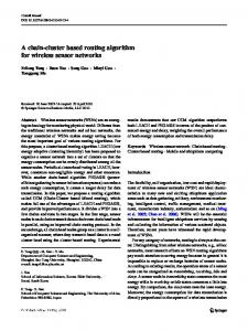
The basic communication problem may be posed as conveying source data with the highest fidelity possible without exceeding an available bit rate, or it may be posed as conveying the source data using the lowest bit rate possible while maintaining a specified reproduction fidelity. In either case, a fundamental trade-off is made between bit rate and signal fidelity. The ability of a source coding system to suitably choose this trade-off is referred to as its coding efficiency or rate distortion performance. To represent a signal in the digital domain, it has to go through a number of steps as shown in Figure(1) which are described in turn [9].
generally irreversible and results in loss of information. It therefore introduces distortion into the quantized signal that cannot be eliminated. One of the basic choices in quantization is the number of discrete quantization levels to use. The fundamental trade-off in this choice is the resulting signal quality versus the amount of data needed to represent each sample [13]. C. Encoding Encoding is a digital symbol processing operation in which the digital form of the information is changed for improved communication. In general, encoding contains many different processes, such as ciphering, compression, and error control coding. One of the main purposes of encoding is compressing information. By using data compression we can reduce the disk space needed to store data in a computer. In the same way we can decrease the required data rate on the line to a small fraction of the original information data rate. We could, for example, use very short codes for the most common characters instead of the full seven-bit ASCII code. Rarely needed characters would use long codes and the total data rate would be reduced [14]. III.
Data compression is the art of reducing the number of bits needed to store or transmit data. There are two types of compression, lossy and lossless. Lossy compression reduces file size by eliminating some unneeded data that will not be recognized by the human after decoding, this is often used in video and audio compression. Losslessly compressed data on the other hand, can be decompressed to exactly its original value. This is important because if a file is lost even a single bit after decoding, will mean the file is corrupted [15]. These steps can be used to reduce the transmission overhead attributed to data transmission. WSN devices are universal and applicable to many sensing and control applications, making the characteristics of various presented datasets wide and varied.
A. Sampling [10]
IV.
A digital signal is formed from an analogue signal by the operation of sampling, quantizing, and encoding. The analogue signal, denoted x(t), is continuous in both time and amplitude. The result of the sampling operation is a signal that is still continuous in amplitude but discrete in time. Such signals are often referred to as sampled-data signals. A digital signal is formed from a sampled data-signal by encoding the timesampled values onto a finite set of values. B. Quantization Quantization is the division of a quantity into a discrete number of small parts, often assumed to be integral multiples of a common quantity. The oldest example of quantization is rounding off, which was first analysed by Sheppard [11] for the application of estimating densities by histograms [12]. Quantization makes the range of a signal discrete, so that the quantized signal takes on only a discrete, usually finite, set of values. Unlike sampling (where we saw that under suitable conditions exact reconstruction is possible), quantization is
DATA COMPRESSION
A RITHMETIC CODE
Arithmetic coding is a technique for coding that allows the information from the messages in a message sequence to be combined to form a single bit stream. A code word is not used to represent a symbol of the text. Instead it uses a fraction to represent the entire source message [15].The technique allows the total number of bits sent to asymptotically approach the sum of the self information of the individual messages (recall that the self information of a message is defined as log2 (1/Pi )). In the following discussion we assume the decoder knows when a message sequence is complete either by knowing the length of the message sequence or by including a special endof-file message. We will denote the probability distributions of a message set as p(1), . . , p(m), and we define the accumulated probability for the probability distribution as in equation 1
www.ijacsa.thesai.org
f (j) =
j−1 X
p(i)(j = 1, ...., m).
(1)
i=1
219 | P a g e
(IJACSA) International Journal of Advanced Computer Science and Applications, Vol. 6, No. 6, 2015
Fig. 1: Sampling, quantizing, and encoding.
The main idea of arithmetic coding is to represent each possible sequence of n messages by a separate interval on the number line between 0 and 1.The occurrence probabilities and the cumulative probabilities of a set of symbols in the source message are taken into account. The cumulative probability range is used in both compression and decompression processes. In the encoding process, the cumulative probabilities are calculated and the range is created in the beginning. While reading the source character by character, the corresponding range of the character within the cumulative probability range is selected. Then the selected range is divided into sub parts according to the probabilities of the alphabet. Then the next character is read and the corresponding sub range is selected. In this way, characters are read repeatedly until the end of the message is encountered. Finally a number should be taken from the final sub range as the output of the encoding process. This will be a fraction in that sub range. Therefore, the entire source message can be represented using a single fraction. To decode the encoded message, the number of characters of the source message and the probability/frequency distribution are needed [16] .
A. Position Any location on Earth is described by two numbersits latitude and its longitude. If a ship wants to specify position on a map, these are the coordinates they would use. Actually, these are two angles, measured in degrees, minutes of arc and seconds of arc. These are denoted by the symbols ( , , ) e.g. 35 43 9 means an angle of 35 degrees, 43 minutes and 9 seconds. A degree contains 60 minutes of arc and a minute contains 60 seconds of arcand you may omit the words of arc where the context makes it absolutely clear that these are not units of time. Calculations often represent angles by small letters of the Greek alphabet, and that way latitude will be represented by l (lambda, Greek L), and longitude by f (phi, Greek F) [17]. B. Velocity Velocity is the rate of change of the position of a ship, equivalent to a specification of its speed and direction of motion e.g. (60 km/h to the north). The applicable range in the marine environment would be between 0 and 75 Km/h. C. Humidity
V.
B ENEFITS OF THE P ROPOSED S YSTEM
Our proposed work is a real world environmental sensor application surveillance system in a marina environment. The purpose of our network is to collect environmental information from different ships. Each ship has a box for AIS and a VHF transceiver. A number of sensors will be placed on the ship to get useful information of(Position,Velocity,Humidity, Temperature, Wind speed, Wind direction, Barometric Pressure, Salinity,Depth, and PH). This data is then sent through a mobile ad-hoc network of ships by multi hop over VHF radio to a destination computer where the accumulated collected data, can be processed for end user applications (Accuracy of Weather information, up to date depth information, and etc.). Because of the low bandwidth available , it is a beneficial for WSNs to employ data compression algorithms. Low-complexity and small size data compression algorithms for sensor networks are therefore essential. The proposed algorithm; Average Marine Data Compression (AMDC) solves this problem by reducing the amount of data presents in the network channel.
VI.
S UMMARIZATION AND A NALYSIS OF M ARINE S ENSOR DATA
The most important sensors applied in our proposed sensor network are as follows:
Humidity of air is a function of both water content and temperature. The relative humidity of an air-water mixture is defined as the ratio of the partial pressure of water vapour (H2O) in the mixture to the saturated vapour pressure of water at a given temperature. The applicable range in the marine environment would be between 0 and 100 %. D. Temperature Temperature is a comparative objective measure of hot and cold. It is measured, typically by a thermometer, through the bulk behaviour of a thermometric material, detection of heat radiation, or by particle velocity or kinetics. It may be calibrated in any of various temperature scales, Celsius, Fahrenheit, Kelvin, etc. The applicable range of air temperature in the marine environment would be between -50◦ and 50◦ C. While sea water temperature is inclusive between -2◦ and 36◦ C. E. Wind Speed Wind speed is the measure of motion of the air with respect to the surface of the earth covering a unit distance over time. The applicable range would be between 0 and 110 mph. F. Wind direction Wind direction is an indicator of the direction that the wind is heading and is usually measured in a degree between 0 and 360.
www.ijacsa.thesai.org
220 | P a g e
(IJACSA) International Journal of Advanced Computer Science and Applications, Vol. 6, No. 6, 2015 G. Barometric pressure Barometric pressure (also known as atmospheric pressure) is the force exerted by the atmosphere at a given point. It is known as the weight of the air. A barometer measures barometric pressure. Measurement of barometric pressure can be expressed in millibars (mb) or in inches or millimetres of mercury (Hg). The applicable range would be between 800 and 1100 mb. H. Salinity Salinity precisely measures the total dissolved salt content of ocean or brackish water. The applicable range would be between 0 and 44%. I. Depth A depth sensor measures sea level close to the shore and in the deep ocean. The highest applicable reading in the marine environment is about 10,925 m. J. PH A PH sensor measures sea and ocean water acidity in the range between 0 and 14 . A neutral reading would be around 7.
For each of the sensors mentioned previously we have set the extreme lower and upper limits of the sensors readings likely to be found in the marine environment as well as the level of accuracy required to represent each reading. This would enable us during the quantization process to reduce the number of bits required for representing the readings of each sensor limited to the predefined ranges and accuracy steps within those ranges. Table II below shows each sensor measurement and the corresponding step level required. VII.
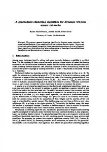
is used to specify whether the latitude is north or south. Ships Longitude [18] is also represented in degrees and tenths of a degree, measured in degrees east or west of the Greenwich Meridian. Values reverse at the international dateline. Tenths are obtained by dividing the number of minutes by 6, and disregarding the remainder (Ignoring seconds). Coding is done with four digits, with the leading (hundreds) figure coded as 0 or 1. The first three digits are actual degrees, the last digit for tenths of a degree. Code 142◦ 55 as 1429 (142◦ is coded as is, 55 divided by 6 is 9, the remainder is ignored); code 60◦ 31 as 0605 (60◦ is coded as 060, 31 divided by 6 is 5, the remainder is ignored); code 9◦ 40 as 0096 (9◦ is coded as 009, 40 is coded as 6); code 0◦ 16 as 0002 (0◦ is coded as 000, 16 is coded as 2). Longitude can vary from 0◦ (coded 0000 on the Greenwich Meridian) to 180◦ (coded 1800 on the dateline). Quadrant of the globe (Qc) is used to specify whether the longitude is east or west. Quadrant of the globe [18] varies according to your position with respect to the equator (0◦ latitude) and the Greenwich Meridian (0◦ longitude). If you are north of the equator (north latitude), Qc is coded as 1 when east of the Greenwich Meridian (east longitude), or as 7 when west of the Greenwich meridian; If you are south of the equator (south latitude), Qc is coded as 3 when east of the Greenwich meridian, or as 5 when west of the Greenwich meridian as shown in Figure(2). For positions on the equator, and on the Greenwich or 180th meridian, either of the two appropriate figures may be used.
Fig. 2: Positioning according to quadrant of the globe
Q UANTIZATION OF M ARINE S ENSOR DATA
All the bit calculations were done according to the quantization rules in a straightforward manner where we use the range of readings for each sensor and the required steps within that range to calculate the exact number of possible readings that should be represented as binary bits. The only exceptions are the positioning readings (longitude and latitude) which were represented so as to reduce even more the bit representation required. In all cases linear quantisation is used. able I shows the lower and upper bound ranges for each sensor and the derived no of bits required representing each sensor reading. Ships latitude [18] is represented in degrees and tenths of a degree, measured in terms of degrees north or south of the equator. Latitudes are determined using standard shipboard methods i.e. a GPS receiver. Tenths are obtained by dividing the number of minutes by 6, and disregarding the remainder (Ignoring seconds). Coding is done with three digits; the first two digits are actual degrees, the last digit for tenths of a degree. Code 46◦ 41 as 466 (46◦ is coded as is, 41 divided by 6 is 6 5/6, 5/6 is disregarded); 33◦ 04 as 330 (33◦ is coded as is, 04 divided by 6 is 4/6 which is disregarded and coded as 0 in this case); 23◦ 00 as 230. Latitude can vary from 0◦ (coded 000) to 90◦ (coded 900). Quadrant of the globe (Qc)
VIII.
T HE PROPOSED COMPRESSION ALGORITHM
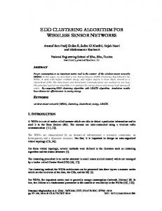
The model of the proposed algorithm, the Average Marine Data Compression (AMDC) consists of three phases: 1. Quantizer: For our marine application, the data gathered from sensors are predictable, therefore it is essential to quantize the data to reduce the amount of bits needed to represent each reading in the binary representation. 2. Average Reading value (AR): It is calculated by summing the four readings after the current reading (Ri) from the sensors, then the deviation from the first reading is calculated as shown in equation 2 .
AR = Ri −
4 X
Ri+j .
(2)
j=1
3. Arithmetic Coder: It calculates the arithmetic code for both (Ri) and (RA) values. After compression, the data is transmitted to the channel, Figure 3 shows this scheme.
www.ijacsa.thesai.org
221 | P a g e
(IJACSA) International Journal of Advanced Computer Science and Applications, Vol. 6, No. 6, 2015
TABLE I: Sensor reading ranges and the derived no of bits required to represent each reading Parameters
Lower value
Upper value
Quantized Representation
Position Longitude Latitude
0 0
90 180
12 13
Velocity Speed Direction
0 0
76 8
7 3
Weather temperature
-50
50
8
Weather humidity
0
100
7
Wind direction
0
360
9
Wind speed
0
110
7
Water temperature
-2
36
6
Pressure barometric
800
1100
9
Salinity
0
44
7
Depth
0
10925
14
PH sensor
6.9
7.2
2
TABLE II: Sensor accuracy step level required Sensor Measurement
Accuracy Step Level
Ship speed Air temperature Air humidity Wind Direction Wind speed Water temperature Sea Level Pressure Salt level in water Depth of water PH level
0.5 km/h 0.5 deg. C 1.0 % 1.0 deg 1.0 m/s 0.5 deg. C 0.5 mb 0.5% 1.0 Meter 0.1
Fig. 3: AMDC Proposed Model
The Measured sensor readings are converted to a binary representation taking into account the quantization of each sensor reading as shown in Table I. Quantization readings are represented by N bits in an analogue to digital converter (ADC), where N is the resolution of the ADC .
compression algorithm particularly suitable for the limited storage and computational resources of a wireless sensor network node. We have simulated the algorithm and used it on our marine data that was obtained from an AIS live system [19], [20]. Note some of the readings were obtained using interpolation. we compare between our proposed algorithm and the Arithmetic coding algorithm and evaluate the performance of the algorithm using the compression ratio metric for the compressed data at the originator node. We obtain the compression ratio 90.11 % and 89.25 % for the two data samples respectively. X.
IX.
E XPERIMENT
In this paper, we propose a specific data formatting for the data gathering application and compress this data to reduce the size of data transmission for sensor nodes over the marine network channel. However, in our proposed MANET over VHF radio frequencies, the transmission bandwidth used is 9.6 Kb/Sec. By reducing data size less bandwidth is required for sending and receiving data. The data compression is one effective method to utilize limited resources of WSNs, therefore its crucial to compress the data before sending over the transmission media. We have simulated a lossless data
R ESULT AND COMPARISON
The scheme presented can be implemented on sensors in a WSN. In our application we used 11 sensors, which sense values once each minute. According to our quantization method in Table I, we have 104 samples for one reading for the whole 11 sensors. The performances of the schemes were analysed according to the number of bits required to transmit the acquired data and the compression ratio. During simulation, attention was focused only on the bits required to compress the data. Sets of data were considered, representing the (Position, velocity, humidity, temperature, wind speed, wind direction, barometric pressure, salinity, depth and PH) values collected
www.ijacsa.thesai.org
222 | P a g e
(IJACSA) International Journal of Advanced Computer Science and Applications, Vol. 6, No. 6, 2015 during 15 minutes in the marine environment. Considering the acquisition time of 15 minutes, the sensor should acquire one values for each minute. For 11 sensors we have 11 readings, the total transmitted bits for the compressed data is 2085, while the total amount of compressed values is of 206 bits. For the two examples discussed (data1, data2) the results can be seen in Figure 4.
in order to gather important sensor data is a promising research field to overcome the high cost burden of satellite communications currently in place. But on the other hand due to bandwidth limitations of the VHF channel, minimizing transmission data redundancy overhead is essential for efficient use of the transmission channel. For our marine application, the predictability of gathered sensor data makes it beneficial to quantize the data to reduce the amount of bits needed to represent each reading in the binary representation. Applying this quantization in conjunction with the proposed compression algorithm (AMDC) has proved affective data compression rates in comparison with the major known compression methods. R EFERENCES [1]
[2]
[3]
Fig. 4: comparison between Arithmetic code and AMDC The metric used to compute the performance of the data compression algorithm is the compression ratio and is defined as the ratio between the size of the compressed file and the size of the source file as shown in Equation 3 : CR = 100 ∗ (1 − CSize /OSize )
[4]
[5]
[6]
(3) [7]
where CR (Compression ratio) , CSize (Compression size) and OSize (Orginal size) respectively, the size of the compressed and the uncompressed bit stream.
[8]
Table III summarizes the results obtained by applying the proposed compression algorithm in contrast with applying arithmetic code compression for two data sets that represent two different input streams of marine sensor data. The table shows clearly that the proposed (AMDC) algorithm outperforms arithmetic code in compression rate for both data sets applied.
[10]
TABLE III: Comparison Ratio for Data1 and Data2
[12]
Arithmetic code compression
Proposed AMDC compression
Data 1
80.04%
90.11%
Data 2
79.23%
89.25%
[9]
[11]
[13] [14] [15] [16]
[17]
XI.
C ONCLUSIONS
MANET networks in the marine environment using VHF technology available on the majority of ships and vessels
[18] [19]
N. Kimura and S. Latifi, “A survey on data compression in wireless sensor networks,” in Information Technology: Coding and Computing, 2005. ITCC 2005. International Conference on, vol. 2. IEEE, 2005, pp. 8–13. J. G. Kolo, S. A. Shanmugam, D. W. G. Lim, L.-M. Ang, and K. P. Seng, “An adaptive lossless data compression scheme for wireless sensor networks,” Journal of Sensors, vol. 2012, 2012. R. Mohsin and J. Woods, “Performance evaluation of manet routing protocols in a maritime environment,” in Computer Science and Electronic Engineering Conference (CEEC), 2014 6th. IEEE, 2014, pp. 1–5. A. K. Maurya, D. Singh, and A. K. Sarje, “Median predictor based data compression algorithm for wireless sensor network,” International Journal of Smart Sensors and Ad Hoc Networks, vol. 1, no. 1, pp. 62–65, 2011. C. M. Sadler and M. Martonosi, “Data compression algorithms for energy-constrained devices in delay tolerant networks,” in Proceedings of the 4th international conference on Embedded networked sensor systems. ACM, 2006, pp. 265–278. T. Bordley, “Linear predictive coding of marine seismic data,” Acoustics, Speech and Signal Processing, IEEE Transactions on, vol. 31, no. 4, pp. 828–835, 1983. M. Schmalz, G. Ritter, and F. Caimi, “Data compression techniques for underwater imagery,” in OCEANS’96. MTS/IEEE. Prospects for the 21st Century. Conference Proceedings, vol. 2. IEEE, 1996, pp. 929–936. D. F. Hoag, V. K. Ingle, and R. J. Gaudette, “Low-bit-rate coding of underwater video using wavelet-based compression algorithms,” Oceanic Engineering, IEEE Journal of, vol. 22, no. 2, pp. 393–400, 1997. “Digital signals - sampling and quantization.” [Online]. Available: http://www.rs-met.com/documents/tutorials/DigitalSignals.pdf H. Johansson, “Sampling and quantization,” Academic Press Library in Signal Processing: Signal Processing Theory and Machine Learning, vol. 1, p. 169, 2013. W. Sheppard, “On the calculation of the most probable values of frequency-constants, for data arranged according to equidistant division of a scale,” Proceedings of the London Mathematical Society, vol. 1, no. 1, pp. 353–380, 1897. R. M. Gray and D. L. Neuhoff, “Quantization,” Information Theory, IEEE Transactions on, vol. 44, no. 6, pp. 2325–2383, 1998. A. Kondoz, “Sampling and quantization,” Digital Speech: Coding for Low Bit Rate Communication Systems, Second Edition, pp. 23–55. T. Anttalainen, Introduction to telecommunications network engineering. Artech House, 2003. M. Mahoney, “Data compression programs,” 2008. S. Kodituwakku and U. Amarasinghe, “Comparison of lossless data compression algorithms for text data,” Indian journal of computer science and engineering, vol. 1, no. 4, pp. 416–425, 2010. D. P. Stern, “Latitude and longitude,” Web page, NASA, Goddard Space Flight Center, Greenbelt, Maryland, vol. 17, 2004. U. D. O. COMMERCE. F. Inc., “Live marine traffic.” [Online]. Available: https://www.marinetraffic.com
www.ijacsa.thesai.org
223 | P a g e
(IJACSA) International Journal of Advanced Computer Science and Applications, Vol. 6, No. 6, 2015
[20]
“Tonbridge-weather.” [Online]. weather.org.uk/home.htm
Available:
http://www.tonbridge-
www.ijacsa.thesai.org
224 | P a g e