Mar 16, 2004 - Abstract. The prevalence of the IEEE 802.11b technology has made Wi-Fi based Audio/Video (AV) conferencing applications a viable service.
An Adaptive Delay and Synchronization Control Scheme for Wi-Fi Based Audio/Video Conferencing Haining Liu and Magda El Zarki Donald Bren School of Information and Computer Sciences University of California, Irvine, CA 92697 {haining, magda}@ics.uci.edu
Abstract The prevalence of the IEEE 802.11b technology has made Wi-Fi based Audio/Video (AV) conferencing applications a viable service. However, due to the “best-effort” transport service and other unpredictable factors such as user mobility, location and background traffic, the transport channel behavior often fluctuates drastically. It thus becomes rather difficult to configure an appropriate de-jitter buffer to maintain the temporal fidelity of the AV presentation. We propose in this paper an adaptive delay and synchronization control scheme for AV conferencing applications over campus-wide WLANs. Making use of a distributed timing mechanism, the scheme monitors the synchronization errors and estimates the delay jitters among adjacent Media Data Units (MDUs) in real-time. It piece-wisely controls the equalization delay to compensate for the delay jitters experienced by MDUs in a closed-loop manner. We investigate the performance of the proposed scheme through trace-driven simulations. We collected network traces from a production campus-wide IEEE 802.11b WLAN by emulating real conferencing sessions. Simulation results show that the scheme is capable of dynamically balancing between synchronization requirements and latency requirements in all scenarios. Small synchronization phase distortions, low MDU loss percentages and low average end-to-end delay can be achieved simultaneously.
1
In particular, compared with solutions using a static setting, the proposed scheme is able to achieve a reduction of around 100ms in end-to-end delay with the same amount of MDU losses under some media-unfriendly situations.
keywords: Wi-Fi, AV conferencing, adaptive delay and synchronization control
1
Introduction
The tremendous success of the IEEE 802.11b technology and the popularity of portable computing units (e.g., PDAs) have made Wi-Fi based real-time multimedia applications a reality. For example, with Wi-Fi based campus-wide broadband wireless coverage, end users can enjoy on-demand streaming of audio or video, or even engage in mobile AV conferencing using PDAs on the go within the covered area. However, due to the lack of QoS support from the network infrastructure, end users often suffer from poor quality assurance. A typical packet-based AV conferencing application works as follows. Audio and video signals are periodically captured at the sender side, fragmented into MDUs, encapsulated and transported across the network in succession to the receiver. Received MDUs are then decoded and rendered to the end users in real-time. As such, different from data applications that usually only concern data fidelity, AV conferencing applications also require the preservation of the temporal fidelity, which calls for appropriate synchronization control to restore the original temporal orderings among the transmitted MDUs, and the stringent control of the latency between the two communications parties to ensure acceptable user interactivity. Without guaranteed transport performance, currently the only viable solution to the synchronization control is to employ a receiving buffer at the receiver end to equalize the variable network delay that each MDU experienced. Since the bandwidth consumption of an AV conferencing session is much smaller than the nominal bandwidth provided by IEEE 802.11b technology (a few hundred kbps vs. up to 7.7 Mbps), one may argue that a small fixed buffering delay is sufficient enough to 2
absorb the delay variations. Unfortunately, our tracing experiment has revealed that such a simplistic approach could easily fail in a real situation [23]. Ideally, an adaptive buffering scheme that is able to dynamically balance between the delay and synchronization requirements could tackle the problem. When the channel condition permits, it reduces the latency as much as possible if synchronization performance allows; when the channel condition degrades, it increases the buffering delay to compensate for the delay jitters. However, due to the random access MAC protocol [1] and the complication introduced by mobility, a transport channel over IEEE 802.11b WLAN often shows “chaotic” characteristics. This makes the design of the adaptive scheme a rather challenging task. We propose in this paper an adaptive delay and synchronization control scheme for Wi-Fi based AV conferencing applications. We focus on campus-wide IEEE802.11b WLANs that are generally capable of supporting low-latency multimedia applications. The proposed scheme enables localized control at the receiver side by employing a distributed timing mechanism. Based on real-time monitored synchronization errors and real-time statistical estimation of the delay jitters among adjacent MDUs, the scheme piece-wisely adjusts the equalization delay to compensate for the delay jitters. We collect network traces from a real campus-wide IEEE 802.11b WLAN by emulating real conferencing sessions, and investigate the performance of the proposed scheme. Through simulations, we show that the proposed scheme is capable of dynamically balancing between synchronization and latency requirements. Overall, small phase distortions, low MDU loss percentages and low average end-to-end delays can be achieved simultaneously using the proposed scheme.
2
Related Work and Motivation
Previous work on application-level synchronization control mostly focused on networked singleobject multimedia applications, specifically, on VoIP applications [2]-[7]. It is worth noting that 3
all proposed schemes rely on a globally synchronization clock and their effectiveness has a close relationship with the “quasi-stationary” property of the wireline network delay process. There have only been a few reported attempts aimed at low-latency multi-object applications such as AV conferencing. In [8], a scheme assuming “no-delay-variation” service for the audio from the underlying network is proposed for wireless PCS systems. It lacks generality due to this unrealistic assumption on the Internet. In [9] and [10], an algorithm facilitating the occurrence of synchronization events is designed for an FDDI/Ethernet based AV teleconferencing system. Because of the relatively small network delay variations, the proposed scheme sets a stiff discard boundary for each stream to achieve intra-stream synchronization, and consequently, the impact on synchronization distortion caused by both MDU loss and MDU skipping is overlooked. In our previous works [11]-[12], we propose a more generic control scheme for AV conferencing applications over wireline IP networks, however, the solution also assumes a “quasi-stationary” characteristic of the network delay process. The end-to-end channel behavior for real-time applications in the emerging campus-wide WLANs remains an unexploited territory. Most previous measurement studies focused on the domain-level performance, e.g., overall network usage and user mobility patterns [13][14][15][16]. The first attempt to investigating the packet loss and delay characteristics of IEEE 802.11b wireless link is reported in [17], but unfortunately, the analysis was performed at the MAC level, and the tracing was carried out without any background traffic. The motivation for the work proposed in this paper is to provide an adaptive delay and synchronization control scheme for Wi-Fi based AV conferencing applications, particularly those over campus-wide WLANs. The proposed solution originates from our solution for wireline applications but deviates from it by taking into consideration the particular difficult characteristic of the wireless transport channel—“non-stationary”. We collect realistic network traces from a production campus-wide WLAN to gain better understanding of the channel behavior, and investigate the
4
performance of the proposed solution using the real traces.
3
An Application-Level QoS Driven Control Scheme
The proposed scheme employs a distributed timing mechanism, monitors the application-level QoS performance at the receiver side, and regulates the equalization delay by adjusting the virtual clock to balance between synchronization requirements and delay requirements.
3.1
Distributed Timing
Our proposed scheme makes use of a distributed timing model. At first, the mechanism attaches the generation time, which records the original temporal information of the presentation, to each MDU sent out from the sender (e.g. via a transport protocol such as RTP). At the receiver side, the mechanism introduces a virtual clock in addition to the actual time. The virtual clock is initialized upon the receipt of the first MDU and runs at the same pace as the real clock of the end system. By doing so, the receiver has two time events for each arrived MDU: the original generation time tg , which is sampled at the source, and the arrival time Ta which is sampled according to the virtual clock. The receiver can simply converts the generation time into the scheduled playout time (i.e., tg ≡ Tg ), compare the generation time with the arrival time and modify the playout time Tp of the MDUs, to achieve an adaptive timeline. Note that Ta , Tg and Tp all reference the local vitual clock. In the meantime, the receiver can adjust the clock (slowdown or speed up) based on the observation of the arrival events. For example, if the scheduled playout time of an MDU is always later than its arrival time, the virtual clock can be sped up to decrease the buffering delay. Obviously, by using such a distributed timing mechanism, the adaptive control can be safely performed by only sampling the local clock.
5
3.2
Application-Level QoS Metrics
Low-latency networked multimedia applications, such as AV conferencing, typically have to fulfill three types of requirements to provide satisfactory performance for end users. First, the temporal inconsistency in presenting the periodically generated MDUs, which is defined as Synchronization Phase Distortion (SPD)[20], has to be controlled below a certain threshold value. Since audio and video are usually tightly coupled in an AV conferencing session, both intra-stream and inter-stream inconsistencies have to be taken into consideration. Second, the loss of data fidelity has to be limited to a tolerable level, otherwise, the resultant information loss is detrimental to the user perceived quality. Finally, the end-to-end delay, which is also defined as latency, has to be confined to an acceptable level to enable real-time interactivity. We therefore define the objective performance measures for AV conferencing as follows. The SPD is jointly evaluated by the Root Mean Square Error (RMSE) of the inter-sample time of the MDUs in one stream (audio/video intra-stream) and the RMSE of the playout time of the closest corresponding data units among two streams (inter-stream). Using the distributed timing mechanism, the intra-stream SPD is given by v u Ni £¡ ¢ ¡ ¢¤2 uP u Tpi (n) − Tpi (n − 1) − Tgi (n) − Tgi (n − 1) t τi = n=2 . Ni − 1
(1)
where Ni denotes the total number of MDUs played out in stream i. Similarly, the inter-stream SPD between audio and video is given by v u Na £¡ ¢ ¡ ¢¤2 u P u Tpa (m) − Tpv (n) − Tga (m) − Tgv (n) t m=1 , τa,v = Na
(2)
where the audio stream is the reference stream and MDU n of the video stream corresponds to MDU m of audio stream. We evaluate the final data loss of a particular media stream i by MDU loss ratio li , which is given by li =
(Mi − Ni ) , Mi 6
(3)
where Mi denotes the total number of MDUs generated in stream i. Note that the MDUs skipped by the adaptive control are also considered as lost ones. The end-to-end delay is defined as the time from when an MDU enters the transport channel to the instant that it is taken from the equalization buffer, i.e. the average latency of stream i is given by
di =
Ni h³ P
n=1
´i i (n) + π i (n) πnet buf Ni
(4)
i (n) and π i (n) denote the network delay and the buffering delay experienced by MDU where πnet buf
n played out in stream i respectively. We do not consider the time that it takes for end systems to collect, encode, decode and render the media data as it is usually a constant component of the end-to-end delay on a specific computing unit (as discovered in [18] )and can be compensated for in a real implementation.
3.3
Closed-Loop Synchronization Control
Motivated by the discovery that the human perception system can tolerate a certain amount of rendering jitter (i.e., phase distortion) of multimedia objects [19][20], we propose to partition the arrival time of the MDUs in the virtual timing space into two regions–“playout” and “discard”, as illustrated in Figure 1. To allow more late MDUs to be rendered, the scheduled playout deadline is extended by a discard boundary δi for each MDU in the stream i. Then depending on which region the MDU n falls into, it is either played out in a controlled manner or is simply discarded. Pseudocode in Figure 2 illustrates the playout time determination process. Note that we apply a smoothing factor αi to minimize the SPD caused by consecutive late arrivals.1 Due to the extension of the discard boundary, potentially large SPD could result. We therefore need to exert tight intra-stream synchronization control for each stream. We use a sliding window to 1
The choice of α is media and implementation dependent. For audio, Reference [5] describe an approach to smooth
out the rendering. For video, the smoothing factor is constrained by the hardware and the driver’s API interface.
7
monitor the resultant SPD and the loss ratio of each stream in real-time. Based on the monitoring results, the receiver maintains satisfactory synchronization performance piecewisely by regulating the buffering delay through virtual clock adjustment. For instance, if either the observed SPD or the MDU loss ratio has exceeded the threshold value, the receiver increases the buffering time by slowing down the virtual clock to allow more “in-time” arrivals. The measured SPD of stream i, τˆi , over a sliding window, is given by v u Wi £¡ ¢ ¡ ¢¤2 uP u Tpi (n) − Tpi (n − 1) − Tgi (n) − Tgi (n − 1) t τˆi = n=2 ¯i − 1 W
(5)
¯ i is the maximum window size. Wi ranges from 2 to W ¯ i, where Wi is the current window size and W and it is incremented by 1 upon the playout of each MDU. The measured loss ratio ˆli is defined as ˆli = ψi , ¯i W
(6)
where ψi is the loss count within the current monitoring window. In addition to the intra-stream control for each stream, a proper inter-stream synchronization control has to be performed to maintain the correct relative temporal positioning between audio and video objects in an AV conferencing session. That is, the inter-stream SPD needs to be controlled below the threshold value throughout the session. Due to the fact that audio quality is more sensitive to delay variations for the human perception system, we assign the audio stream as the master stream, which dominates the inter-stream synchronization control, and apply the inter-stream synchronization constraint to the video stream. For each MDU of the video stream, after the playout time determination process, its playout time is rechecked with a closest available audio MDU to satisfy the inter-stream synchronization requirements. Pseudocode in Figure 3 illustrates such an MDU-by-MDU enforcement process, where τ¯a,v denotes the threshold value of the inter-stream SPD between audio and video. The overall control scheme integrating both intrastream and inter-stream synchronization control is shown in Figure 4. The scheme originates from 8
our previous work for wireline scenarios. However, in order to cope with the “non-stationary” property, we employ an on-line status estimator for each stream which serves to measure the delay jitters and estimate the status of the underlying transport channel in run-time. The estimation is used jointly with the monitored SPD and loss ratio for the clock adjustment decision. We detail the clock adjustment process in the next section.
4 4.1
Clock Adjustment Principles and Challenges
Recall that using the virtual timing model, adjusting the virtual clock is equivalent to adjusting the buffering delay to “equalize” the variable delay jitters. In our scheme, the adjustment is driven by the observed arrival events and the measured SPD and loss ratio, and appears in the form of expanding/shortening the playout duration of one MDU, or proactively skipping received MDUs (see Algorithm 1). The essence of the adjustment is illustrated in Figure 5. We consider that the probability distribution of the network delays conforms to a generic “heavy-tail” shape, which is typical in “best-effort” packet switched networks. Then the scheme is aimed at adjusting the equalization delay (i.e., the clock offset between the generation clock at the sender side and the virtual clock at the receiver side, which is denoted as oi ) to accommodate for the delay variations experienced by most MDUs. For stream i, based on the observation of its MDU arrival events over a monitoring window, the equalization delay is either reduced (by ∆i1 ) to reduce the end-to-end latency if the synchronization performance permits, or increased (by ∆i2 or ∆i3 ) to maintain the synchronization performance if excessive synchronization errors (in the form of excessive SPD value or loss ratio) have occurred. Since the clock adjustment is solely driven by the observed synchronization errors, i.e., the scheme purposely behaves in a greedy way to satisfy the synchronization requirement, we
9
can expect for the adjustment to occur mainly at the tail portion of the probability distribution. If the network delay process shows a characteristic of “quasi-stationary”, i.e., the probability distribution observed over different monitoring periods stays roughly the same, over a relatively large time scale (e.g., 30s), we can derive a closed form expression for the adjustment amount by making a few simple assumptions (c.f. [12]). However, in a WLAN scenario, the network delay process can by no means be assumed to be stationary due to a number of random factors involved in the transport process such as channel fading, backgournd traffic and user mobility. The probability distributions of network delays over two contiguous monitoring windows could be drastically different as illustrated in Figure 5. This phenomena consequently poses two challenges. First, we need to take into consideration this dynamic characteristic while deriving the clock adjustment amount. Second, the clock adjustment has to be performed conservatively in case the scheme is too agile, i.e., overreacting to the state transition of the transport channel, which usually leads to frequent clock adjustments and introduces nonnegligible synchronization errors. We derive the expression for the clock adjustment amount in the next subsection.
4.2
Clock Adjustement Parameters
As discussed in the above subsection, we need to enforce a very conservative principle on clock adjustments while dealing with WLAN transport channels, particularly on the clock speed-up. Only when the measured synchronization errors (SPD and MDU losses) are all zero over the maximum monitoring window, do we consider to speed up the clock to reduce the latency. We employ an on-line status estimator (as illustrated in Figure 4) and estimate the worst-case arrival situation based on the observed MDU arrival events. We show the concept in Figure 6. The worst-case estimation approach is inspired by the 3-sigma rule in statistical process control, which is used to judge if the production process is out of control [21]. Only when a relatively stable
10
status of the channel is detected over a period of time (i.e. for each MDU n of stream i that arrived in the monitoring window, we have observed Tai (n) < Tgi (n)), we estimate the worst possible MDU arrival time and derive the speed-up amount thereafter.2 We first obtain the sample value of the delay jitter between two consecutively generated MDU n by S i (n) =
£¡
¢ ¡ ¢¤ Tai (n) − Tai (n − 1) − Tgi (n) − Tgi (n − 1) .
(7)
We then recursively update the moving range of the delay jitter, which is the average of the differences between two adjacent sample points, to approximate the standard deviation [22], i.e. σjitter =
Wi X ¯ i ¯ ¯(S (n) − S i (n − 1)¯ /(n · 1.128),
¯ i. Wi = 2, ..., W
(8)
n=2
When a clock speed-up adjustment is found to be necessary, we first get the average gap between the arrival time and the scheduled playout time of all MDUs in the monitoring window, Gavg , by ¯
Gavg
Wi X £ i ¤ ¯ i. = (Tg (n) − Tai (n) /W
(9)
n=1
Then the adjustment amount ∆i1 is calculated by ∆i1
¾ £ i ¤ i = min max (Tg (n) − Ta (n) , (Gavg + 3 · σjitter ) . ½
¯i n∈W
(10)
Note that the amount is guaranteed to be smaller than the largest gap observed over the maximum monitoring window, an additional procedure used to ensure a conservative adjustment. When the measured SPD exceeds the threshold value, the clock needs to be slowed down by ∆i2 to allow more in-time MDU arrivals to reduce the distortion. We denote the monitoring window size of this moment as Wi and calculate ∆i2 as follows. Since the adjustment is triggered by the observed SPD value, intuitively, it usually happens on the tail portion of the delay p.d.f. We therefore can safely assume that every MDU of stream i within the monitoring window Wi arrived 2
Some may argue that the estimate is not accurate when delay jitters are not normally distributed. However, in
our case, the approach provides a fairly good approximation with very low computing cost.
11
later than the scheduled playout time but ahead of the discard boundary δi (a worst-case scenario), and uniformly distributed within this range. If we denote X i (n) = Tai (n) − Tgi (n), then X i (n) conforms to a uniform distribution within [0, δi ]. Applying the Central Limit Theorem, with a probability of 1, the mean square error of the SPD we observed over Wi satisfies (W ) i X ¡ ¢ £ i ¤ 2 ¯i − 1 ≤ / W X (n) − X i (n − 1) i=2
h
(Wi − 1) µ + 3.1 · σ
i ¡ p ¢ ¯i − 1 , Wi − 1 / W
(11)
£ ¤2 where µ and σ 2 are the expected value and the variance of random variable X i (n) − X i (n − 1) . We assume that over two adjacent monitoring periods, the difference between two observed delay
probability distributions can be approximated by a “tail shift” as illustrated in Figure 7. This assumption can safely hold as long as the probability distribution has a “heavy tail”. Under this e i assuming the network delay is an i.i.d. assumption, we first obtain the adjustment amount ∆ 2 e i (oi → oei ), we should expect process. That is, after the clock is slowed down by ∆ 2 i ¡ h p p ¢ ¯ i − 1, ¯ i − 1 ≥ µ0 + 3.1 · σ/ W (Wi − 1) µ + 3.1 · σ Wi − 1 / W
(12)
h 0 i2 0 0 0 where µ and σ 2 are the expected value and the variance of random variable X (n) − X (n − 1) , h i 0 e i . On the basis of a worst and similarly X (n) conforms to a uniform distribution within 0, δi − ∆ 2 case situation, we can get
e i2 ∆
=
Ã
1−
s
Wi − 1 ¯i − 1 W
!
· δi .
(13)
We then estimate the shifting amount based on the MDU arrival events observed. We employ an agile exponentially-weighted moving average (EWMA) filter [22] to recursively estimate the delay jitters. The filter has the form E i (n) = 0.1 · E i (n − 1) + 0.9 · S i (n),
(14)
where E i (n) is the newly generated estimate based on MDU n’s arrival, E i (n − 1) is the prior estimate and S i (n) is the current observation obtained by applying Equation 7 to MDU n’s arrival. 12
When a clock slow-down is triggered, we simply treat the most recent estimate as the projected shifting amount. As such, if MDU n is the most recently arrived MDU, we obtain ∆i2 by e i2 . ∆i2 = E i (n) + ∆
(15) 0
In accordance with this adjustment, the clock offset now becomes oi . If it is the measured loss ratio that has exceeded the threshold value, we need to slow down the clock by ∆i3 to constrain the MDU losses over the next monitoring window within the threshold value. However, in the WLAN scenario, it is possible that the MDU losses observed during a short period of time could be solely caused by the poor channel quality. In this case, increase the buffering delay in the application layer is not necessary at all. Therefore, we need to differentiate the MDU losses caused by the channel itself from the MDU losses caused by skipping. We use a heuristic approach to tackle this problem. A counter is used in the status estimator to record the number of the MDUs which arrived but were skipped during a monitoring period. If the counter’s value is zero when a clock slowdown request is triggered by excessive observed losses, we simply ignore such a request. If the counter’s value is nonzero, we enable the clock slowdown and obtain e i assuming an i.i.d. delay ∆i3 by applying the same “tail-shifting” assumption. We first obtain ∆ 3
process, i.e., the following equation ¾ ½ £ i ¤ i i e max Ta (n) − Tg (n) − ∆3 W n∈Wi ½ ¾ = i ¯i £ ¤ W max Tai (n) − Tgi (n) − δi
(16)
n∈Wi
should hold to ensure that the measured loss ratio over the next window should not exceed the threshold value. We hence obtain ¶ µ £ i ¤ Wi Wi i i e + δi · ¯ ∆3 = max Ta (n) − Tg (n) 1 − ¯ n∈Wi Wi Wi ≈ δi .
13
(17)
If the most recent estimate is E i (n), then ∆i3 is obtained by e i3 . ∆i3 = E i (n) + ∆
5
(18)
Performance Evaluation
In this section, we investigate the performance of the proposed scheme. We collect delay traces by emulating real AV conferencing sessions on a production WLAN, and study how the end-to-end transport channel behaves in different scenarios. We then apply the proposed scheme and run simulations off-line. The synchronization performance and delay equalization control behavior are evaluated.
5.1
Trace Collecting and Simulation Parameters
For AV conferencing applications over WLAN, we consider two possible scenarios: the session is carried out either between stationary parties or between mobile parties. In order to make the results comparable, we set up the experiments by emulating two application scenarios separately in the same WLAN. The two tracing sessions, however, are run simultaneously. One is between two stationary parties, and the other one is between two mobile parties. Details of the trace collection process are described in a longer version of this work in [23]. We simulate the AV application using the G.723.1 codec for audio and MPEG-4 codec for video. The encoded data are transported over the RTP/UDP/IP protocol stack. Altogether we collected 10 traces (5 between stationary parties, referred to as S1-5, and 5 between mobile parties, referred to as M1-5). We list these 10 traces and some related details in Table 1. With the aid of the network management system, each trace was collected while the network was moderately loaded. We choose the simulation parameters of the proposed scheme according to the performance threshold values reported in previous work [19], [20] and [25]. For the audio, we set the τ¯a (intra14
stream SPD threshold) to be 3ms. The smoothing factor αa is set to be 10ms, which in turn guarantees that each rendered audio MDU lasts for at least 30-10=20 ms (c.f. [5] for a scaling playout algorithm of audio). Recall that in the proposed scheme, we differentiate the MDU loss which is introduced by the transport channel, from the MDU skipping, which is caused by proactive intra-stream synchronization control. The real MDU losses are not counted during the monitoring process. We hence set the maximum tolerable loss ratio over a monitoring window, ¯la , to be 0.01, which indeed only considers MDU skipping and is smaller than the real tolerable loss ratio threshold (usually 3% - 5%). With regard to the uniform distribution assumption that is used to derive the adjustment amount, we set the discard boundary, δa , to be 25ms, a relatively large value. For the video, τ¯v is set to be 5 ms, and the smoothing factor αv is set to be 16.667 ms, a common refreshing interval on modern displays. Similar to the choices of audio, ¯lv is set to be 0.01, and δv is set to be 60ms. τ¯a,v , the maximum allowed inter-stream skew between audio and video, is set to be 80 ms. We set the maximum sliding window size of both audio and video to be 1000, which guarantees a sufficiently large sampling space for monitoring. In order to further reduce the SPD and MDU skipping that are caused by initial adjustments of an adaptive control, we apply a 100ms initial buffering delay to each stream. That is, the virtual clock is started 100ms later after the first audio MDU is received.
5.2
Simulation Results
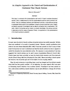
We first study how a static scheme, i.e., setting a static equalization delay, performs given the different delay traces we collected. Figure 8 and Figure 9 show the total resultant media MDU loss ratios when different equalization delay values are applied to each trace. It can be seen that, during the same time period, sessions between mobile parties generally experience larger delay variations than those carried between stationary parties do. However, we also observe that, due to
15
different background traffic, the transport channel between stationary parties sometimes behaves no better than that between mobile parties (e.g., S4 vs. M2, M3, M5), though the network is similarly loaded. This undoubtedly proves the unpredictability of the transport channel behavior on a WLAN. Figure 8 and Figure 9 also imply that all traces have a “heavy-tail” characteristic of their probability distributions. When the equalization delay increases, the MDU loss ratio curve slowly decreases to the limit, which is set by the channel losses. Figure 8 and Figure 9 also corroborate our analysis in Section 1 that a static setting of equalization delay cannot cope well with the unpredictable channel behavior. We observe that, in some cases (e.g., M1 and M4), the transport channels behaved very poorly that even a large static equalization delay (over 400 ms) can not completely compensate for the delay variations. Next, we apply the proposed adaptive scheme to the 10 traces, and investigate the synchronization and delay control performance. The results are summarized in Table 2. We observe that the proposed scheme clearly demonstrates the capability to balance in real-time the synchronization requirements and the latency preference. When the transport channel yields relatively small delay variation and small MDU loss percentage ( as shown by trace S1 and S3), the intra-stream and inter-stream synchronizations are perfectly maintained while the end-to-end delay is maintained at a fairly low level. When the transport channel introduces larger delay variation and more MDU losses (as exemplified by trace S2, M2, M3, S4, S5 and M5), the proposed scheme regulates the end-to-end delay adaptively to compensate for the larger delay jitters, and reduces the MDU skipping as much as possible while keeping the synchronization distortions below the threshold values. Eventually, the SPD values, the resultant MDU loss ratios and the end-to-end latency are all kept at an acceptable level.3 When the transmission performance of the channel further deteriorates, e.g., as shown by trace M1 and M4, a large percentage of MDUs experience network delay values 3
Performance rating is obtained by referencing [19], [20] and [25].
16
larger than 400ms, and a nonnegligible amount of MDUs are lost, the proposed scheme still strives to maintain a fairly good synchronization performance and a tolerable average end-to-end latency ( δi then 2:
discard MDU n
3: end if 4: if Tai (n) − Tgi (n) ≤ δi then 5:
if Tpi (n − 1) == Tgi (n − 1) then
6:
Tpi (n) ← max Tai (n), Tgi (n)
�
�
7:
end if
8:
if Tpi (n − 1) > Tgi (n − 1) then
9: 10:
h
Tpi (n) ← max Tai (n), Tgi (n), Tpi(n − 1) + Tgi (n) − Tgi (n − 1) − αi end if
11: end if
Figure 2: Playout time determination algorithm
21
i
Algorithm 2 Inter-Stream Synchronization Constraint Enforcement 1: for MDU n in the video stream do 2:
pick the closest available corresponding MDU m in the audio stream
3:
eint ← Tpv (n) − Tpa (m) − Tgv (n) − Tga (m)
4:
if |eint | ≤ τ a,v then
5:
Tpv (n) ← Tpv (n)
6: 7: 8: 9: 10:
h
i
h
else if eint > τ a,v then Tpv (n) ← max else
h�
i
�
Tpa (m) + Tgv (n) − Tga (m) + τ a,v , Tav (n)
i
Tps (n) ← Tpa (m) + Tgv (n) − Tga (m) − τ a,v end if
11: end for
Figure 3: Inter-stream synchronization control
22
Determine Playout Time Master
Put into Monitoring Window and Calculate Synchronization Errors
Adjust the Virtual Clock If Necessary
Decode & Play Back
Status Estimator Virtual Clock Status Estimator Determine Playout Time
Adjust Playout Time under Inter-Stream Synchronization Constraint
Put into Monitoring Window and Calculate Synchronization Errors
Adjust the Virtual Clock If Necessary
Decode & Play Back
Slave
Figure 4: A closed-loop delay and synchronization control scheme
23
Probability Clock offset = (π ��
+ � )
Discard boundary
−∆� +∆�� � Delay
o
o + δ
Figure 5: Clock adjustemnt vs. delay distribution
24
Observed Probability
−∆� Delay
�
−∆� Estimated worst case
Figure 6: Clock speed-up based on the worst-case situation
25
�
T�
o
�
� T� �
�
o�
�
�
� �/ ∆ �� ∆
� o
�
� �
o� + δ�
E (n )
�
o � + δ�
Figure 7: Clock slow-down on a shifting tail
26
S1 S2 S3 S4 S5
0.25
0.2
Loss Ratio (%)
Loss Ratio (%)
0.2
S1 S2 S3 S4 S5
0.25
0.15
0.1
0.15
0.1
0.05
0.05
0
0 50
100
150
200
250
300
350
400
450
50
500
a.
100
150
200
250
300
350
400
450
Equalization Delay (ms)
Equalization Delay (ms)
Audio
b.
Video
Figure 8: Resultant loss ratios for sessions between stationary parties using static equalization delay
27
500
M1 M2 M3 M4 M5
0.25
0.2
Loss Ratio (%)
Loss Ratio (%)
0.2
M1 M2 M3 M4 M5
0.25
0.15
0.1
0.05
0.15
0.1
0.05
0
0
50
100
150
200
250
300
350
400
450
500
50
Equalization Delay (ms)
a.
100
150
200
250
300
350
400
450
Equalization Delay (ms)
Audio
b.
Video
Figure 9: Resultant loss ratios for sessions between mobile parties using static equalization delay
28
500
d
c
b
e
a
d
f
Cumulative Probability
Cumulative Probability
0.95 (274.26~304.26)sec (304.26~334.26)sec
c
b
e
1
1
a
f
0.95 (274.26-304.26)sec (304.26-334.26)sec
(334.26~364.26)sec
(334.26-364.26)sec
(364.26~366.39)sec
(364.26-366.39)sec
(366.39~388.29)sec
(366.39-388.29)sec
0.9
0.9
0
50
100
150
200
250
300
350
400
450
500
0
50
100
150
200
Delay (ms)
a.
250
300
350
400
450
Delay (ms)
Audio
b.
Video
Figure 10: An example operation of adaptive equalization delay adjustment (trace M1)
29
500
Table 1: Collected Network Delay Traces 1-min Avg. Traffic Load
1-min Avg. User Count
before the Tracing (kbps)
before the Tracing
Trace
Start Time
AP1
AP2
AP1
AP2
S1, M1
15:07 March 16, 2004
1200
650
4
3
S2, M2
15:21 March 17, 2004
1420
580
5
3
S3, M3
16:01 March 18, 2004
970
510
5
2
S4, M4
15:30 March 22, 2004
1690
830
7
4
S5, M5
15:16 March 23, 2004
750
620
4
3
30
Table 2: Synchronization and Delay Control Performance Trace S1 M1 S2 M2 S3 M3 S4 M4 S5 M5
Intra-stream SPD (ms)
Audio Video Audio Video
1.1 1.7 3.4 5.1
Audio Video Audio Video
2.6 4.9 3.4 4.8
Audio Video Audio Video
1.0 0.6 2.5 3.7
Audio Video Audio Video
3.5 4.7 3.0 3.7
Audio Video Audio Video
2.9 4.3 3.1 4.9
Inter-stream SPD (ms) 0.8 1.1 2.4 1.3 0.8 0.9 1.6 2.2 1.1 2.9
31
Loss Ratio
End-to-end Latency (ms)
0.008 0.008 0.044 0.047
142.9 142.9 258.7 258.7
0.016 0.016 0.029 0.028
147.1 147.1 178.5 178.5
0.004 0.004 0.02 0.02
62.5 62.5 92.0 92.0
0.025 0.023 0.054 0.043
234.7 234.7 296.1 296.1
0.016 0.023 0.027 0.026
135.2 135.2 190.1 190.1
References [1] M. Heusse, F. Rousseau, G. Berger-Sabbatel, and A. Duda, “Performance anomaly of 802.11b,” Proc. of Infocom 2004, HongKong, March, 2004. [2] R. Ramjee, J. Kurose, D. Towsley, and H. Schulzrinne, “Adaptive playout mechanism for packetized audio applications in wide-area networks,” Proc. of IEEE INFOCOM 1994, Los Alamitos, CA, June, 1994, pp. 680–688. [3] S. B. Moon, J. Kurose, and D. Towsley, “Packet audio playout delay adjustment: Performance bounds and algorithms,” ACM/Springer Multimedia Systems, vol. 5, no. 1, pp. 17–28, Jan. 1998. [4] J. Rosenberg, L. Qiu, and H. Schulzrinne, “Integrating packet FEC into adaptive voice playout buffer algorithms on the internet,” Proc. of Infocom 2000, Tel Aviv, Israel, March 2000. [5] Y. J. Liang, N. F¨arber, and B. Girod, “Adaptive playout scheduling and loss concealment for voice communication over IP networks,” IEEE Transactions on Multimedia, vol. 5, no. 4, pp. 532–543, Dec. 2003. [6] H. Melvin and L. Murphy, “An evaluation of the potential of synchronised time to improve VoIP quality,” roc. IEEE ICC 2003, Anchorage, Alaska, USA, May, 2003. [7] M. Narbutt and L. Murphy, “VoIP playout buffer adjustment using adaptive estimation of network delays,” Proc. of International Teletraffic Congress ITC-18, Berlin, Germany, AugustSeptember, 2003. [8] H. Liu and M. E. Zarki, “Delay and synchronization control middleware to support real-time multimedia services over wireless PCS networks,” in IEEE JSAC, vol. 17, no. 9, pp. 1660–1672, 1999. 32
[9] C. Liu, Y. Xie, M. Lee, and T. Saadawi, “Multipoint multimedia teleconference system with adaptive synchronization,” IEEE JSAC, vol. 14, pp. 1422–1435, Sept. 1996. [10] Y. Xie, C. Liu, M. J. Lee, and N. Saadawi, “Adaptive multimedia synchronization in a teleconference system,” ACM/Springer Multimedia Systems, vol. 7, no. 4, pp. 326–337, 1999. [11] H. Liu and M. E. Zarki, “A synchronization control scheme for real-time streaming multimedia applications,” Proc. 13th Packet Video Workshop, Nantes, France, April, 2003. [12] H. Liu and M. E. Zarki, “On the adaptive delay and synchronization control for video conferencing over the internet,” Proc. of ICN 2004, Guadeloupe, French Caribbean, March, 2004. [13] D. Tang and M. Baker, “Analysis of a local-area wireless network,” Proc. of Mobicom 2000, Boston, Massachusetts, August 2000. [14] D. Kotz and K. Essien, “Analysis of a campus-wide wireless network,” Proc. of Mobicom 2002, Atlanta, Georgia, September 2002. [15] A. Balachandran, G. M. Voelker, P. Bahl, and P. B. Rangan, “Characterizing user behavior and network performance in a public wireless LAN,” Proc. of ACM SIGMETRICS 2002, Marina del Rey, California, June 2002. [16] M. Balazinska and P. Castro, “Characterizing mobility and network usage in a corporate wireless local-area network,” Proc. of MobiSyS 2003, San Francisco, California, May, 2003. [17] C. Hoene, A. Gunther, and A. Wolisz, “Measuring the impact of slow user motion on packet loss and delay over IEEE 802.11b wireless links,” Proc. of WWLN 2003, Germany, October 2003. [18] I. Kouvelas, V. Hardman, and A. Watson, “Lip synchronization for use over the internet: Analysis and implementation,” Proc. of IEEE Globecom 1996, London, UK, November, 1996. 33
[19] R. Steinmetz and C. Eagler, “Human perception of jitter and media synchronization,” Internal Report #43.9310, IBM European Networking Center, Heidelberg, Germany, 1993. [20] R. Steinmetz, “Human perception of jitter and media synchronization,” IEEE JSAC, vol. 14, pp. 61–72, Jan. 1996. [21] D. W. B. G. Barrie Wetherill, Statistical Process Control: Theory and Practice, 1st ed. London, New York: Chapman and Hall, 1991. [22] N. M. Kim, B, “Mobile network estimation,” Proc. of Mobicom 2001, Rome, Italy, Jun. 2001. [23] H. Liu and M. E. Zarki, “Adaptive Delay and Synchronization Control for Wi-Fi Based AV Conferencing,” in Proc. of Qshine 2004, Dellas, TX, October, 2004. [24] I. JTC1/SC29/WG11, MPEG-4 video verification model 10.0, Feb., 1998. [25] D. Miras, “A survey on network QoS needs of advanced internet applications,” Working Document of Internet 2 QoS Working Group, 2002. [26] Y. Ishibashi, S. Tasaka, and H. Ogawa, “A comparison of media synchronization quality among reactive control schemes,” Proc. of Infocom 2001, Anchorage, Alaska, USA, April, 2001.
34