IEEE TRANSACTIONS ON FUZZY SYSTEMS, VOL. 10, NO. 2, APRIL 2002
247
An Adaptive Neuro-Fuzzy System for Automatic Image Segmentation and Edge Detection Victor Boskovitz and Hugo Guterman
Abstract—An autoadaptive neuro-fuzzy segmentation and edge detection architecture is presented. The system consists of a multilayer perceptron (MLP)-like network that performs image segmentation by adaptive thresholding of the input image using labels automatically pre-selected by a fuzzy clustering technique. The proposed architecture is feedforward, but unlike the conventional MLP the learning is unsupervised. The output status of the network is described as a fuzzy set. Fuzzy entropy is used as a measure of the error of the segmentation system as well as a criterion for determining potential edge pixels. The proposed system is capable to perform automatic multilevel segmentation of images, based solely on information contained by the image itself. No a priori assumptions whatsoever are made about the image (type, features, contents, stochastic model, etc.). Such an “universal” algorithm is most useful for applications that are supposed to work with different (and possibly initially unknown) types of images. The proposed system can be readily employed, “as is,” or as a basic building block by a more sophisticated and/or application-specific image segmentation algorithm. By monitoring the fuzzy entropy relaxation process, the system is able to detect edge pixels. Index Terms—Adaptive thresholding, fuzzy entropy, image segmentation, neuro-fuzzy system, self-organizing system.
I. INTRODUCTION
I
MAGE segmentation is the technique of decomposing an image into meaningful parts, or objects [1]–[3]. It results in a segmented image, where each object is labeled in a way that facilitates the description of the original image so that it can be interpreted by the system that handles the image. In general, the classification of an image’s pixels as belonging to one of the “objects” (i.e., classes) composing the image is based on some common feature(s), or resemblance to some pattern. In order to determine which are the features that can lead to a successful classification, some a priori knowledge or/and assumptions about the image are usually required. It is due to this fact that the best results are obtained by segmentation algorithms “tailored” for specific applications (but which will perform poorly on applications other than the one they were designed for). The majority of the segmentation algorithms produce two level, or “object and background” segmentation. While such a result is appropriate for some of the ‘classical’ image processing
Manuscript received May 15, 2001; revised July 20, 2001 and September 4, 2001. The authors are with the Department of Electrical and Computer Engineering, Ben-Gurion University of the Negev, Beer-Sheva 84105, Israel (e-mail:
[email protected]). Publisher Item Identifier S 1063-6706(02)02968-5.
applications such as the automatic image analysis of documents or industrial parts, it is not satisfactory for applications dealing with more complex scenes, where several objects have to be detected. In this paper, we propose a system capable to perform multilevel segmentation of images in an automatic/unsupervised way. No a priori assumptions whatsoever are made about the image (type, features, contents, stochastic model, etc.). Such an “universal” algorithm is most useful for applications that are supposed to work with different (and possibly initially unknown) types of images (e.g., searching for images on the Internet or in the photo archive of a magazine). The proposed system can be readily employed, “as is,” or as a basic building block by a more sophisticated image segmentation algorithm (that incorporates additional “knowledge” into different parts of the system). The proposed neuro-fuzzy segmentation system is self-organizing. It consists of a multilayer perceptron (MLP)-like network that performs image segmentation by adaptive thresholding of the input image using labels automatically pre-selected by a fuzzy clustering technique. The proposed architecture is feedforward, but unlike the conventional MLP, the learning is unsupervised. The output status of the network is described as a fuzzy set. Fuzzy entropy is used as a measure of the error of the segmentation system. Because this measure handles only one aspect of the quality of the segmentation, and because no satisfactory quality measures were proposed in the literature, the results are analyzed mainly by visual inspection and comparison with results obtained by other algorithms. One of the main roadblocks toward full automation of the segmentation system is the problem of automatically choosing the correct number of labels. This parameter, of crucial importance to most labeling methods, is usually very hard to determine automatically, and in most cases it is left as a parameter which has to be provided by the user. Some methods of employing cluster validity measures to solve this problem were tested, and some preliminary results are presented in this paper. The paper is organized as follows. First, the image segmentation problem is defined (Section II). Section III contains a survey on prior research that is most closely related to the present work. In particular, applications of several fuzzy logic (mostly fuzzy clustering) and neural networks techniques to the field of image segmentation are reviewed. Some fuzzy logic terms and concepts involved in the development of the proposed system are reviewed in Section IV. A detailed description of the proposed system follows (Section V). Relevant results are presented in Section VI. Finally, Section VII ends the paper with several conclusions drawn from the design of and the work with the proposed system.
1063-6706/02$17.00 © 2002 IEEE
248
IEEE TRANSACTIONS ON FUZZY SYSTEMS, VOL. 10, NO. 2, APRIL 2002
II. THE IMAGE SEGMENTATION PROBLEM Image segmentation is a process that partitions an image into the different objects composing it. The objects are sets of points that naturally form a group in their measurement space. In the segmented image, each object is labeled in a way that reflects the “actual structure” of the data and facilitates the description of the original image so that it can be interpreted by the system that handles the image further. Depending on whether spatially separated objects of the same kind have to be labeled the same or not, the image segmentation problem may be regarded as a classification problem or a clustering one, respectively. Several authors (e.g., [4]) employed the following formal definition of image segmentation. Formal definition: Let denote the grid of all the pixels in the image, i.e., the set of all the pairs: . where and are the number of rows and columns of the matrix representing the image, and be a uniformity (or homogeneity) predicate which aslet signs the value TRUE or FALSE to a nonempty subset of , depending only on properties related to the value of the pixels also has the property that given a subset of in the subset. , say , and a subset of , say implies . always that A segmentation of the grid for a uniformity predicate is a partition of into disjoint nonempty subsets such that: with ( every pixel 1) must be in one, and only one, segment); is connected (i.e., composed of con2) tiguous grid points); for (the segments should 3) be uniform, in terms of the chosen ); when is adjacent to . 4) In what regards constraint 2) above, the reader familiar with the problem might argue that some of the segmentation algorithms produce nonconnected (or nonconvex) segments (e.g., classical thresholding algorithms). On the other hand, these nonconvex segments may be treated as sets of several connected segments that were given the same label. More important, it should be noted that the definition above only defines what are the constraints on a possible segmentation of an image, and not what a correct segmentation of an image is. III. NEURAL, FUZZY AND HYBRID APPROACHES TO IMAGE SEGMENTATION The image segmentation approaches are too numerous to be accounted for in a single text [1], [2], [4]. Here, the main neural, fuzzy and hybrid approaches to image segmentation will be enumerated. A. Neural Network Approaches to Image Segmentation With the aim of obtaining adaptive image processing, researchers have tried to employ neural network (NN) approaches [5], [6]. Here, the basic objective is to emulate the human vision processing system which is highly robust and noise insensitive and hence can be applied even when information is ill defined and/or defective/partial. Image segmentation problems can be
approached as either classification or clustering problems (depending on the application at hand), both of which are ‘natural’ applications of existing NNs. In addition, NN-based algorithms have been developed to solve the image segmentation problem by emulating different existing approaches (relaxation, edge detection, etc.). Several NN image processing models have been proposed, of most interest to this research being those which are auto-adaptive (or self-organizing) [7]–[10]. When supervised training is possible, the most straightforward and popular approach to NN-based image segmentation is to use a feedforward, back-propagation trained MLP. A comprehensive analysis of the performance of such a system and its comparison with other image segmentation methods is presented in [11] and [12]. To overcome the limitations imposed by supervised training, some methods to produce image segmentation using unsupervised NNs have also been developed, such as the Kohonen’s learning vector quantization (LVQ) network [7], [13] and the Adaptive Resonance Theory (ART) networks, developed by Carpenter and Grossberg [14], [15]. Besides these originally unsupervised NNs, some ways were found to add a self-organizing capability to supervised NNs [9], [16]. B. Fuzzy Logic Approaches to Image Segmentation An increasing number of fuzzy logic approaches that treat (i.e., understand, represent and process) the images, their segments and features as fuzzy sets have been investigated in the last decade [4], [9], [11], [17], [18]. This is also true for the specific task of image segmentation, which in this context can be seen as the process of imposing a crisp structure on the fuzzy data. This task can be carried out by different fuzzy clustering algorithms. For example, Hall et al. [11] used the Fuzzy -Means (FCM) algorithm to segment MR images, where each pixel is a 3-D vector consisting of different features yielded by the MRI system. Using the pixel coordinates as input features in addition to the intensity values also makes sense (although no mention of it was found in the literature). The cluster validity problem in this context was addressed by Bensaid et al. [19], by incorporating a validity measure into the FCM algorithm. With the aim of accounting for the local characteristics of images, Tolias and Panas [20] developed an algorithm that combines the results of performing the FCM algorithm on a set of different resolution realizations of the original image. Also of interest is their implementation, reported in the same paper, of the Possibilistic -Means (PCM) clustering algorithm [21]. Another approach to image segmentation using fuzzy logic is based on the minimization of the fuzzy entropy of the image. Because this approach is most closely related to the present work, we briefly address the question of “Why fuzzy entropy minimization results in image segmentation?” A segmented image can be seen as a union of crisp sets (e.g., pixels belonging to object A or B or background), therefore, the original image can be seen as a union of fuzzy sets describing the relative membership of its pixels (based on their gray level or some other feature) to the different crisp sets (see also Section IV-A). It follows that the segmentation problem might be seen as the problem of matching the fuzzy set describing a given image to the crisp set that most
IEEE TRANSACTIONS ON FUZZY SYSTEMS, VOL. 10, NO. 2, APRIL 2002
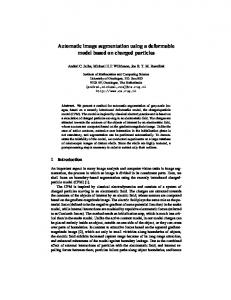
Fig. 1. Histogram based fuzzification (adapted from [17]).
likely describes the segmented image. This matching can be obtained by minimizing the fuzziness measure of the given image (the fuzziness measure being the distance to the closest crisp set or the fuzzy entropy). Different fuzzy entropy functions have been employed by researchers for object-background segmentation [9], [10], [22]. The most widely used definitions are presented in Section IV.B. Detailed accounts of fuzzy entropies and their application in image segmentation can be found in [23] (maybe for the first time) and in [24] (most recently). C. Hybrids (Fuzzy NNs) for Image Segmentation Some NNs that incorporate fuzzy clustering strategies have been developed. Bezdek et al. [25] proposed a fuzzy Kohonen clustering network by integrating the FCM algorithm into the learning method of the traditional Kohonen network. Davis et al. [26] proposed the implementation of the FCM algorithm by means of a feedforward, back-propagation trained NN. Lin et al. [27] integrated the FCM algorithm into a 2-D Hopfield NN (called by them Fuzzy Hopfield NN), to obtain unsupervised classification of MR brain images based on the within-class scatter matrix. IV. FUZZY THEORY ISSUES RELEVANT TO THIS WORK
249
expresses an average measure of ambiguity in associating an element to a certain fuzzy set, the second one measures the fuzziness of a partition of the data set and is usually employed as a validation measure of a clustering solution. Here, the fuzziness measures of fuzzy sets will be discussed. Most researchers agree that such a measure should satisfy the following properties, originally proposed by De Luca and Termini [29]: • (or other unique minimum) iff or (if is crisp); a unique maximum iff ; • where is a sharper version of , i.e., • for for • where
, where
is the complement of
.
fuzziness measure of fuzzy set ; membership function (in the fuzzy set); supporting points of the fuzzy set . Before proceeding, a note should be made on the analogy between the terms of fuzziness and entropy. De Luca and Termini [29] observed that fuzziness is a measure of uncertainty, much like entropy is in the field of thermodynamics. They also observed that although nonprobabilistic, the fuzziness of a fuzzy set is a measure of the information contained by it, just like probabilistic entropy is in the field of information theory. This analogy stuck in the fuzzy literature. Therefore, in the rest of this work the terms: “fuzziness,” “measure of fuzziness,” and “fuzzy entropy” will be used interchangeably. There are several types of such measures proposed in the literature [29]–[31]. The most common types are as follows. 1) Distance Measures: Based on the distance between a fuzzy set and either its nearest ordinary set (defined below), or [31]. In general, given a fuzzy set , its its complement nearest ordinary (crisp) set is defined as the set where the memberships are as follows:
A. Histogram Based Image Fuzzification with intensity levels availGiven an image of size , it may be regarded as an array able for each of its pixels of fuzzy singletons whose value of membership denotes the degree to which they posses some property/feature (e.g., brightness, edginess, smoothness), or the extent to which they belong to an image subset (e.g., object, skeleton, contour) [18]. Thus, a gray level image can be seen as a fuzzy partition into certain subsets/classes (e.g., “dark pixels,” “bright pixels,” “pixels belonging to object A,” etc.) as shown in Fig. 1. B. Fuzziness Measure or Fuzzy Entropy Uncertainty either due to vague descriptions, inaccurate measurements, or to random occurrence can be described by means of fuzzy sets theory [28]. In terms of fuzzy sets theory this kind of uncertainty, when measured over a given data set, is called the fuzziness measure. At this point, a slight distinction between fuzziness measures of fuzzy sets and fuzziness measures of fuzzy partitions should be made. While the first one
if if
(1)
The index of fuzziness based on the distance to it is (2) denotes the distance (usually the norm of order where ) between the two sets, is the length of the data set and is the order of the distance used. In particular, when Hamming ), the index of fuzziness (called distance is employed (i.e., in this case the linear index of fuzziness) is given by:
(3)
250
IEEE TRANSACTIONS ON FUZZY SYSTEMS, VOL. 10, NO. 2, APRIL 2002
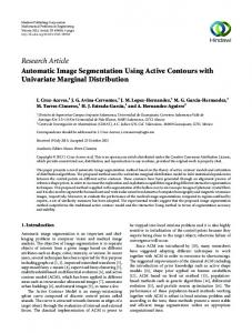
Fig. 2. General flowchart.
When Euclidean distance is employed, (2) gives the quadratic index of fuzziness. Its explicit form becomes
(4)
The fuzziness measures based on the distance to the fuzzy complement have the following general form:
(5)
IEEE TRANSACTIONS ON FUZZY SYSTEMS, VOL. 10, NO. 2, APRIL 2002
251
Fig. 3. Block diagram of proposed system.
As , using the Hamming metric for example, allows for the following substitution:
(which has no “palpable” meaning). In this case, the use of a logarithm function would have an unappealing behavior
(6) Yet another fuzziness measure based on distances between sets was introduced by Kosko [30]. It is defined as the ratio and the distance between the distance to the nearest crisp set to the farthest crisp set (7) 2) Entropy-Like Measures: Based on the analogy between fuzziness and entropy, some measures based on the Shannon function from information theory have been proposed. These are not based on distance measures but satisfy the four De Luca–Termini axioms. See the following for an example. 3) Logarithmic Entropy [29]:
(8) 4) Exponential Entropy: Pal and Pal proposed in [23] a new, exponential form of (fuzzy) entropy [(9)], motivated by the following points. • The logarithmic form is not bounded when the membership values approach zero. • The additive property for independent events is not always important. • Regarding the original Shannon function (or replacing in (8) with , the probability of occurrence of ), it is more mathematically sound to relate the igno, which rance (or potential gain in information) to represents the probability of nonoccurrence, than just to
(9)
V. PROPOSED SYSTEM A. Overview of the Proposed System The proposed system consists of a multilayer neural network that performs adaptive, multilevel thresholding of the image using labels automatically preselected by a fuzzy clustering technique. The learning technique employed is self-supervised allowing, therefore, automatic adaptation of the NN. The output status of the network is described as a fuzzy partition. Fuzzy entropy is used as a measure of the error of the system as well as a criterion for determining potential edge pixels. Given an input image, the system is forced to evolve toward a minimum fuzzy entropy state in order to obtain image segmentation. Pixels most affected by the consecutive training iterations (due to the amount of their contribution to the fuzzy entropy of the system) are labeled as edge pixels. B. System Description A general flowchart of the proposed algorithm is depicted in Fig. 2. First, labels are found by applying the FCM algorithm to the image histogram. Then, the information about the labels is employed to build the network’s activation and error functions. The input to a neuron in the input layer is normalized between [0–1], proportionally to the gray value of the correspondent pixel. The image information is first propagated forward using (11) to get the output status of the network. The output value of each neuron lies in the interval [0–1]. Then, the output error
252
IEEE TRANSACTIONS ON FUZZY SYSTEMS, VOL. 10, NO. 2, APRIL 2002
(a)
(c) Fig. 4.
(b)
(d)
Error functions. (a) Histogram of the Panda image (Fig. 9). (b) Partition found by FCM. (c) Fuzzy entropy [(8)]. (d) Linear index of fuzziness [(3)].
is calculated and then back-propagated to update the weights [(14)]. Training continues either until a minimum error or until a maximum number of iterations is reached. The output of the system at this stage constitutes the segmented image. Integrating (summing) the thresholded (binarized) differences between the output at consecutive epochs yields the edge image. Viewed as a system, the proposed algorithm consists of three main processing blocks (Fig. 3): the (fuzzy) error function definition block (A), the adaptive thresholding block (B) and the optional edge detection block (C). 1) Error Function Definition (Block A): The purpose of this stage is to provide the objective error function to be used by the adaptive thresholding stage (for unsupervised training). First, the input image is fuzzified based on its gray-level histogram (see Section IV-A), and then the error function is obtained by determining the contribution of each graylevel to the fuzzy entropy of the partition (any fuzziness measure can be employed). Two such error functions are depicted in Fig. 4. In our study, the FCM algorithm was employed to create a fuzzy partition that properly describes the image, using only the pixel intensity feature. Other clustering algorithms might be used as well, but because that in the case of 1-D data the shape of the cluster boundaries is of no importance, variations of the objective function minimized by the algorithm (such as Fuzzy -Shells or the more general Gustafson–Kessel algorithms) are of no specific interest here. Some test were run using possibilistic clustering, but no significant difference in the cluster boundaries was found, while the more irregular shape of fuzzy sets obtained eventually slowed down the convergence of the system. In order to keep the system totally autonomous, an automatic way to determine , the right number of clusters, is needed. In the proposed system, this was done by iterating the FCM algorithm for a range of hypothesized numbers of clusters and choosing the best option based on a cluster validity measure. Al-
though in general cluster validity measures are not considered very reliable, some of them (e.g., the partition coefficient and the partition entropy, Bezdek [28]) yielded surprisingly good results for some of the test images. This might be partially due to the special nature of the data, which is not common in clustering problems: the data is 1-D and at least one entry exists at each possible point. Still, in general, the problems involved in this choice are (yet) unsolvable, thus leaving this parameter as the only part of the system requiring the (yet) nonreplaceable human intervention. Supposing that someone does rely on one of the cluster validity measures, another decision has to be made: on one hand, the correct can be chosen as the one providing the extremal value for the specific validity measure employed. On the other hand, accepting the fact that different values of might fit the given data (e.g., for segmentation at different detail), a threshold on the validity measure should be chosen below/above which is accepted. There is (yet) no theoretical way to define such a threshold. Attempts to do this are done based on application/data specific heuristics, like how many different ’s are acceptable, or how far can the threshold be from the extremal value of the validity measure. 2) Adaptive Thresholding (Block B): This stage contains the adaptive thresholding system itself, the fuzzy entropy calculation block and the training/tuning algorithm of the adaptive thresholding system. Its inputs are the input image and the error function determined by stage A. and its output is the segmented image. The adaptive thresholding system is based on a self-organizing neural network (Fig. 5). This part of the system is based on the image segmentation system proposed by Ghosh et al. in [9], [10]. They developed a self-organizing MLP that has an inherent unsupervised learning ability. The network architecture proposed by them is similar to the one used in the present work (see Section V-B), except that in their system the outputs of the network were fed back as inputs to the network after the first forward pass. Their system suited only the task of object-
IEEE TRANSACTIONS ON FUZZY SYSTEMS, VOL. 10, NO. 2, APRIL 2002
253
sists of a sigmoid-like function with multiple levels. The multisigmoid is obtained by the superposition of shifted sigmoid functions ( being the number of classes). The rationale behind using such a function was to enable stability around the multiple targeted pixel values. We define the multisigmoid function as (Fig. 7)
(11) where Fig. 5. Network architecture.
Fig. 6. Neighborhood of a pixel. (a) First order neighborhood; (b) Second order neighborhood; (c) Sequence of neighborhoods.
background separation. Furthermore, they assumed that the membership values of the image pixels in the two classes (object and background) attain their maximum at one of the ends of the intensity value range and descend monotonically toward the other end, attaining the value of 0.5 exactly at the middle of the range. In the proposed system, the neuron activation function and the error measuring function were completely modified in order to deal with multilevel segmentation. The network consists of an input layer, an output layer and at least one hidden layer (Fig. 5). Each layer consists of neurons, every neuron corresponding to an image pixel. Each neuron in one layer is only connected to the corresponding neuron in the previous layer and the neurons in its -th order neighborhood (Fig. 6). A neighborhood system over a lattice is defined as (10) , called the -th order neighborhood of , is such where that ; • implies . • There are no connections between neurons in the same layer. The NNs’ weights cannot be randomly initialized or they will alter the input image. In this work, all weights were initialized to 1, but it is also possible to initialize the weights using some kind of weighting window within the neighborhood of each pixel. 3) Activation function: In order to allow more than two stable states of the neuron output (i.e., more than two allowable intensity levels), a special activation function was developed. It con-
step function; thresholds; target level of each sigmoid, will constitute the systems’ labels; steepness parameter; size of the neighborhood, as defined in the previous section. The thresholds and the target values are obtained from the error function, as the graylevels with the maximal and with minimal levels of fuzziness respectively. Because the range of the neuron input levels depends on the number of neurons in the previous layer to which it is connected (the size of the neighborhood), the threshold values are adapted to reflect this dependency (by multiplying them by , the number of input links). 4) Training: The back-propagation algorithm is employed for training [32]. The weights are updated as follows: output layer other layers (12) where total input to the th neuron; weight of link from neuron in one layer to neuron in the next layer; output of the th neuron in the previous layer; error in the network’s output (relative to the desired target image); learning rate. Note: For simplicity we used 1-D indexes in the above equations, the extension to fit the 2-D NN is straightforward. For a multisigmoid as previously defined (13) and the equations for
become
(14)
254
IEEE TRANSACTIONS ON FUZZY SYSTEMS, VOL. 10, NO. 2, APRIL 2002
Fig. 7. Multisigmoid (example). TABLE I EXECUTION TIMES
(a)
(b) Fig. 9.
Fig. 8. “Panda” image and its histogram.
for the output layer and the other layers respectively. 5) Fuzziness measure/Error function: The error function defined at the first stage of the system is evaluated for the image output at each training epoch. As discussed before, the aim of the network is to reduce the degree of fuzziness of the input image. 6) Defuzzification: As it should be understood from the descriptions of the neural network, it is “working” directly on the graylevel values, and not on their fuzzy membership values, as would be the case in a usual fuzzy image processing algorithm. In other words, the network does not change the fuzzy membership values of the pixels in order to reduce the error. Instead, it changes the initial pixel values to values that will decrease the amount of fuzziness, according to the initial fuzzy partition. Thus, the output of the neural network is initially obtained in terms of graylevels, which are then “fuzzyfied” in order to
(a) Synthetic image and its histogram. (b) Noisy version of (a).
determine the error. In the ideal case when the network con, the outputs have only verges with no error at all values who’s membership values are “1” or “0,” defuzzification is not necessary. When the network does not converge completely (whether stopped intentionally or not), the fuzzification of the output image does not result in merely crisp membership values. The information about the membership values of the pixels might be useful for further processing, depending on the application at hand. If crisp labeling is required, a defuzzification stage must be added. For display purposes, the simplest defuzzification method is thresholding the fuzzy partition, so that each pixel is uniquely assigned to the class in which it has the highest membership value. After being assigned to a single class, the pixels can be labeled either with the value of the prototype of their class, or with the value of the prototype weighted by the membership values of the pixels in their class (thus preserving some of the “fuzzy” information). C. Edge Detection (Block C) The edge detection subsystem was added during the research in order to investigate the possibility to exploit the fuzzy entropy information for other applications. This subsystem is based on the assumption that the edge pixels have the most ambiguous values in the image, i.e., they give the largest contribution to the fuzzy entropy of the output image at each iteration. Thus,
IEEE TRANSACTIONS ON FUZZY SYSTEMS, VOL. 10, NO. 2, APRIL 2002
Fig. 10.
255
Cluster validity for the “Panda” image.
Fig. 11. Cluster validity for the synthetic image.
Fig. 12.
Cluster validity for the noisy synthetic image.
these pixels are those that undergo the greatest changes during the training/tuning of the system. Here, the edge image is obtained by monitoring the changes that take place in the pixels’ values between two consecutive iterations and integrating these changes over the whole training period. VI. RESULTS AND DISCUSSION A. Implementation The main stages of the proposed system were implemented in a single C++ program. The edge detection process and the visualization of the results were carried out using the MATLAB environment. The system was tested on over 100 images of different types, as part of various applications under research at our laboratory. Typical execution times on a Pentium III, 733 MHz computer, with 256 MB of RAM can be seen in Table I. Beside the image size, the execution time of the FCM algorithm iterations also depends on the number of clusters. In average, about 50 iterations are needed. This number also depends on the nature of
the data (whether the clusters are well separated or not) and, of course, on the required precision. The execution time of the NN training epochs depends on the image size and the neighborhood size. Theoretically, the number of required epochs depends on the error and activation functions (which in turn depend on the nature of the data), on the learning rate and on the required precision. Practically, the training may usually be stopped after about ten epochs. In most cases, hard thresholding the output at this stage yields satisfactory results. In terms of run-time memory requirements, the main demands are imposed by the neural network. In special, four floating point matrices (neighborhood size multiplied by the size of size of the image) are needed for the two layers of weights and their corresponding updates, and three floating point matrixes of size (the image size) are needed to store the three layers of the network (input, hidden and output). For example, running the algorithm on a 256 256 image and using a 3 3 neighborhood floating point values, which would require more than translates into 10 MB of memory (assuming 4-byte precision is enough for the floating point values).
256
Fig. 13.
IEEE TRANSACTIONS ON FUZZY SYSTEMS, VOL. 10, NO. 2, APRIL 2002
Images of the NNs layers.
B. Error Function Definition 1) Performance of Some Cluster Validity Measures: The performances of several cluster validity measures were studied, in order to test the possibility of using them as an automatic tool for the determination of the number of classes in an image. The cluster validity measures were applied to the partitions, obtained by means of the FCM algorithm, of the image histograms. The results obtained by the cluster validity measure that turned out the best among those tested are demonstrated here on two images. The “Panda” image shown in Fig. 8 is a natural image with three well-defined classes. The synthetic image in Fig. 9 is composed of five classes. In the case of this synthetic image, the validity measures were tested on the initial image containing well-separated classes [Fig. 9(a)], as well as on a noisy version of the image (Fig. 9(b), Gaussian noise, ). The size of the synthetic image is while the size of the “Panda” image is 141 164. 80 Although the research in this regard is far from being complete, some of the preliminary results are shown here in order to give a “flavor” of what can be achieved by using simple cluster validity measures. The performances of three of the cluster validity measures applied to the test images are presented in Figs. 10–12. These cluster validity measures are the Partition Coefficient [(15)], the Average Partition Separability proposed by Baker [(16)], which might be seen a normalized version
Fig. 14.
Histogram of the synthetic image.
of the partition coefficient, and the Partition Entropy [(17)], all of them described by Bezdek in [28]. The figures show the value returned by the cluster validity measures for different (hypothesized) numbers of classes. The values obtained for the “correct” number of classes are highlighted. (15)
(16)
IEEE TRANSACTIONS ON FUZZY SYSTEMS, VOL. 10, NO. 2, APRIL 2002
Fig. 15.
Images of the weight matrices.
Fig. 16.
Segmentation results and comparison.
257
(17) From the analysis of the results of a significant number of tests, in may be concluded that these measures provided surprisingly good results (relative to other applications of cluster validity) when the objects composing an image are well separated in the intensity level space (otherwise it is hard to judge their performance anyway, as even a human cannot decide which is the true number of classes). Thus, they may be useful in some specific applications, such as the automatic inspection of industrial components.
C. The Operation of the Adaptive Thresholding NN The system’s operation will be presented and explained with the help of a synthetic image. In Fig. 13, the states of the input, the hidden, and the output layers are visualized, after the convergence of the NN. The histogram of the original image is shown in Fig. 14. With two exceptions (marked accordingly), all the results presented in this work were obtained using 3 3 window (neighborhood) size. It can be observed that the NN did not converge completely (the error is not zero), as some of the output values still differ from the chosen labels. These ‘stubborn’ output nodes are located at the borders between two adjacent regions (seg-
258
Fig. 17.
IEEE TRANSACTIONS ON FUZZY SYSTEMS, VOL. 10, NO. 2, APRIL 2002
Effects of increasing the size of the neighborhood.
ments). As anticipated, the edge pixels have the most ambiguous values (this fact is exploited by the proposed edge detection subsystem). Note that while the output of the hidden layer might be already regarded as a segmented image, the result of the output layer is significantly more defined (it contains less ambiguous values). The fact that most of the learning takes place at the boundary between image segments can be also seen in the visualization of the weight values after network convergence (Fig. 15). In Fig. 15, the 2-D images of the weight matrixes of the hidden and of the output layer are shown. Because some of the weights have large positive or negative values, the equation shown at the bottom of the page was applied to the weights in order to visualize their values. D. Segmentation Results The comparison between the segmented image obtained by means of the proposed system and some other algorithms is shown in Fig. 16. Fig. 16(c). shows the results of hard-thresholding the image using the thresholds determined by the FCM algorithm. Figs. 16(d)–(f) show the results produced by three algorithms available in the Khoros environment. It can be observed that the proposed system produces much smoother results (less “noisy” regions), which is a desirable feature, even at the price of loosing some information. The results were ob. tained assuming The region growing algorithm used here, which might not be the best one of it’s kind, produced a clearly inferior result in this case, because it gives different labels to separated (nonconvex) regions even if they are of the same kind. Note that due to the good behavior (well defined clusters) of the example, the results obtained by using the FCM algorithm (Fig. 16(c)) and the (Hard) -Means algorithm are almost the same (only a few pixels differ). Fig. 17 shows the effects of increasing the size of the neighborhood. It can be seen that as the neighborhood is increased, better smoothing is obtained, but more detailed information is lost. As a conclusion, when dealing with noisy images the use of a larger neighborhood size is desirable. Otherwise, smaller neighborhoods should be used to obtain more detail. Other parameters, like the type of error function used (partition entropy, linear index of fuzziness, etc.) and the steepness factor of the multisigmoid activation function did not show any significant influence on the outcome of the segmentation algorithm (they do influence the rate of convergence).
Fig. 18.
Noise immunity.
The proposed system was found to be robust to some real life ‘complications’ like the addition of noise, and changing illumination conditions. For example, Fig. 18 shows the segmentation results of some quite heavily noised versions of the Panda image. Fig. 19 shows a darkened version of the Panda image, its histogram and the segmented image. E. Convergence Analysis We could not prove convergence and stability of the adaptive thresholding system analytically, mainly due to the nonconvex nature of the error function and the complexity of the interactions between the neighborhoods in the neural network. Experimentally, the system was found to converge in all the tested cases in the different applications where it was employed (the system was tested with over 100 images). Here, the convergence of the system when applied to the Panda image is visualized in several ways. Fig. 20 shows the convergence of the error. Three plots of the error as a function of the training epoch are shown, each one obtained for a different weight update strategy. The slowest convergence rate was obtained when the learning rate (LR) was kept constant at a certain value. The fastest one was obtained when using the modified momentum method. This method lead to instability when the error was small (see “zoomed” version of this curve in Fig. 21) because the learning rate reached very high values, which causes “vibration” of output values close to the thresholds. Therefore, a compromise
if else
IEEE TRANSACTIONS ON FUZZY SYSTEMS, VOL. 10, NO. 2, APRIL 2002
259
Fig. 19. Invariance with illumination conditions.
Fig. 20.
Convergence of the error.
Fig. 21.
Unstable convergence.
was obtained by bounding the learning rate by a maximal value (the curve in the middle). Fig. 22 shows the phase diagram of the error (the derivative of the error as a function of the error) obtained when training the system with a constant learning rate. It can be observed that the derivative of the error remains negative (thus, the error always decreases) and it decreases (in absolute value) as the error decreases (thus indicating convergence and stability). Another way to observe the convergence of the system is by analyzing the results of the segmentation itself. This is visualized here by either observing the resulting histogram or the obtained image. Fig. 23 shows the histogram of the output image after 10, 100, and 500 training epochs (when applied to the
Fig. 22.
Phase diagram.
Fig. 23.
Histogram convergence.
“Panda” image), clearly indicating the convergence of the pixel values to the chosen labels. F. Edge Detection Results The edge detection subsystem was found to perform poorly compared to some of the better edge detection algorithms existing today, sometimes even worse than the classical, gradient type edge detectors (Prewitt, Sobel, etc.). Yet, the results are good enough to prove the point that the process of fuzzy entropy
260
Fig. 24.
IEEE TRANSACTIONS ON FUZZY SYSTEMS, VOL. 10, NO. 2, APRIL 2002
(a)
(b)
(c)
(d)
Edge detection results. (a) Original image. (b) Proposed algorithm. (c) DRF. (d) Sobel (thresholded).
Fig. 25. Cell image—segmentation (5 levels) and object extraction. The object extraction image is obtained by replacing the labels of the classes assumed to compose the objects of interest by the original values of the pixels.
minimization does provide information about the ‘edginess’ of the pixels in an image, in addition to the segmentation. Furthermore, the algorithm proposed here has the advantage of being totally automatic. Also, some typical post-processing (like edge linking) might enhance its performance. Fig. 24 shows the results of the edge detection subsystem applied to the Panda image [Fig. 24(b)], compared to the results of the (thresholded) Sobel operator [Fig. 24(d)] and of the optimal Difference Recursive Filter (DRF) for edge detection algorithm. This filter, proposed by Shen and Castan [33], is an
Fig. 26.
Segmentation of IR image (four levels).
Fig. 27.
Segmentation (five levels) of a MRI image.
optimal smoothing filter (symmetric exponential filter of infinitely large window size) based on a one step model (a step edge and the white noise) and the multi-edge model. G. Some Results in Different Applications The proposed system was adapted and integrated into several applications under development at our laboratory. Some of the preliminary results were presented previously [34]–[36]. A few examples of results obtained for different types of images are presented in Figs. 25–27.
IEEE TRANSACTIONS ON FUZZY SYSTEMS, VOL. 10, NO. 2, APRIL 2002
261
VII. DISCUSSION AND CONCLUSION An adaptive system for the automatic segmentation of intensity level images was presented in this paper. In order to achieve the ability to robustly perform across the wide diversity of images encountered in real world applications, resemblance to the human visual system was sought during the design of the system. The “heart” of the proposed system, the neural network that performs the adaptive thresholding, is biologically inspired (beyond the simple modeling of artificial neurons): the pyramidal averaging effect, which is a result of its special architecture, is a known feature of the human visual system; also, the learning process based on the minimization of the fuzzy entropy function is a kind of relaxation process, which is typical of physical systems. The FCM algorithm, used to determine the thresholds and the error function, was designed based on human heuristics of what a “good” partition should be like. Although our aim was to concentrate on the research of the concepts described above rather than to achieve optimal segmentation results, the results we obtained are comparable with those of other known methods and sometimes/from certain points of view might even outperform them. In addition, the proposed system has the advantage that it does not require any human expert intervention, nor any a priori information about the input image. In this study, minimization of an image’s fuzzy entropy was employed as the target of an MLP neural network’s training, thus transforming it into an unsupervised training scheme. Obtaining image segmentation by means of reducing the (fuzzy) entropy of the image can be argued “philosophically” considering both the physical and the information theory significance of “entropy.” The segmentation process may be regarded as one that reduces the uncertainty in the image (about the belonging of pixels to objects), as well as one that results in gain of information (about the structure of the image). In addition to using fuzzy entropy as a measure of the error of the segmentation system, this reasoning also led to its use as a criterion for determining potential edge pixels (here it might be interesting to mention the fact that the segmentation and edge detection operations are complementary aspects of the object extraction problem). It was found that some of the “classical” cluster validity measures can be relied upon in some cases (e.g., industrial applications) to automatically choose the number of clusters (segments) that appear in the image. The system provided good results when tested on noisy images (different types of noise with low SNR were tested) and under changing illumination conditions. Convergence of the adaptive thresholding system was not proven analytically, but it was found experimentally in all the (over 100) test cases. The research issues/directions that might provide the greatest benefit are: • Experimenting with clustering algorithms other than the FCM algorithm, in order to find one that can detect ‘small’ clusters (the FCM algorithm tends to form partitions where the number of data points in all the clusters is similar).
Fig. 28. No caption needed.
• Working with more features at the different processing stages (data fusion). The label choosing system (i.e., the clustering algorithm) can be easily adapted to deal with more features, but in the case of the neural network the implementation of this task is less trivial. In this latter case, some changes to the network architecture are probably required (like linking multiple weights in parallel between the neurons, one for each feature), besides adapting the activation and the error functions. Of most importance are the inclusions of color information (RGB, HUV, etc.) and of local features (gradient value, mean local value, etc.). • Conduct multi-resolution analysis (look for segments at different resolutions) either selecting an optimal global or local window sizes or by integrating the results obtained at different resolutions. • Further research on validity and convergence of the segmentation system, especially in difficult real-life images such as Fig. 28. REFERENCES [1] B. Jahne, Digital Image Processing, 2nd ed. New York: Springer-Verlag, 1993. [2] K. Jain, Fundamentals of Digital Image Processing. Upper Saddle River, NJ: Prentice-Hall, 1989. [3] A. Rosenfeld and A. Kak, Digital Picture Processing. New York: Academic, 1982, vol. II. [4] N. R. Pal and S. K. Pal, “A review on image segmentation techniques,” Pattern Recog., vol. 26, pp. 1277–1294, 1993. [5] B. Kosko, Neural Networks for Signal Processing. Upper Saddle River, NJ: Prentice-Hall, 1992. [6] B. J. Krose and P. van der Smagt, An Introduction to Neural Networks, 5th ed. Amsterdam, The Netherlands: Univ. of Amsterdam, 1993. [7] T. Kohonen, Self-Organization and Associative Memory. New York: Springer-Verlag, 1989. [8] R. O. Duda and P. E. Hart, Pattern Classification and Scene Analysis. New York: Wiley, 1973. [9] A. Ghosh, N. R. Pal, and S. K. Pal, “Self-organization for object extraction using a multilayer neural network and fuzziness measures,” IEEE Trans. Fuzzy Syst., vol. 1, pp. 54–69, Feb. 1993. [10] A. Ghosh, “Use of fuzziness measures in layered networks for object extraction: A generalization,” Fuzzy Sets Syst., vol. 72, pp. 331–348, 1995. [11] L. O. Hall, A. Bensaid, L. Clarke, R. Velthuizen, M. Silbiger, and J. Bezdek, “A comparison of neural network and fuzzy clustering techniques in segmenting magnetic resonance images of the brain,” IEEE Trans. Neural Networks, vol. 3, pp. 672–682, Sept. 1992. [12] J. C. Bezdek, L. O. Hall, and L. P. Clarke, “Review of MR image segmentation techniques using pattern recognition,” Med. Phys., vol. 20, pp. 1033–1048, 1993. [13] N. Pal, J. Bezdek, and E. Tsao, “Generalized clustering networks and Kohonen’s self-organizing scheme,” IEEE Trans. Neural Networks, vol. 4, pp. 549–557, July 1993.
262
[14] G. Carpenter and S. Grossberg, “A massively parallel architecture for a self-organizing neural pattern recognition machine,” Comp. Vision Graph. Image Process, vol. 37, pp. 54–115, 1987. [15] S. Hidemoto and J. Toriwaki, “Automatic segmentation of head MRI images by knowledge guided thresholding,” Comp. Med. Imag. Graph., vol. 15, pp. 233–240, 1991. [16] S. G. Romaniuk and L. O. Hall, “Dynamic neural networks with the use of divide and conquer,” Proc. IEEE Int. Joint Conf. Neural Networks, vol. I, pp. 658–663, 1992. [17] H. R. Tizhoosh, Fuzzy Image Processing. Berlin, Germany: SpringerVerlag, 1997. in German. [18] J. C. Bezdek and S. K. Pal, Eds., Fuzzy Models for Pattern Recognition. New York: IEEE Press, 1992. [19] A. M. Bensaid, L. O. Hall, and J. C. Bezdek et al., “Validity-guided (Re)clustering with applications to image segmentation,” IEEE Trans. Fuzzy Syst., vol. 4, pp. 113–123, 1996. [20] Y. A. Tolias and S. M. Panas, “Image segmentation by a fuzzy clustering algorithm using adaptive spatially constrained membership functions,” IEEE Trans. Syst., Man, Cybern. A, vol. 28, pp. 359–369, May 1998. [21] R. Krishnapuram and J. M. Keller, “A possibilistic approach to clustering,” IEEE Trans. Fuzzy Syst., vol. 1, pp. 98–110, May 1993. [22] S. Di Zenzo, L. Cinque, and S. Levialdi, “Image thresholding using fuzzy entropies,” IEEE Trans. Syst., Man, Cybern. Part B, vol. 28, pp. 15–23, Feb. 1998. [23] N. R. Pal and S. K. Pal, “Object-background segmentation using new definitions of entropy,” in Proc. Inst. Elec. Eng., vol. 136, 1989, pp. 284–295. [24] H. D. Cheng, C. H. Chen, H. H. Chiu, and H. Xu, “Fuzzy homogeneity approach to multilevel thresholding,” IEEE Trans. Image Processing, vol. 7, pp. 1084–1086, July 1998.
IEEE TRANSACTIONS ON FUZZY SYSTEMS, VOL. 10, NO. 2, APRIL 2002
[25] J. C. Bezdek, E. C. K. Tsao, and N. R. Pal, “Fuzzy Kohonen clustering networks,” in Proc. Int. Conf. Fuzzy Systems, San Diego, CA, 1992, pp. 1035–1043. [26] J. P. Davis, T. M. Warms, and W. R. Winters, “A neural net implementation of the fuzzy c-means clustering algorithm,” Proc. IEEE Int. Joint Conf. Neural Networks, p. A-953, 1991. [27] J. S. Lin, K. S. Cheng, and C. W. Mao, “Multispectral magnetic resonance images segmentation using fuzzy Hopfield neural network,” Int. J. Bio. Med. Comp., vol. 42, pp. 205–214, 1996. [28] J. C. Bezdek, Pattern Recognition with Fuzzy Objective Function Algorithms. New York: Plenum Press, 1981. [29] A. De Luca and S. Termini, “A definition of non probabilistic entropy in the setting of fuzzy set theory,” Inform. Control, vol. 20, pp. 301–312, 1972. [30] B. Kosko, “Fuzzy entropy and conditioning,” Inform. Sci., vol. 40, pp. 165–174, 1986. [31] R. R. Yager, “On the measure of fuzziness and negation part I: Membership in the unit interval,” Int. J. Gen. Syst., vol. 5, pp. 221–229, 1979. [32] R. P. Lippmann, “An introduction to computing with neural nets,” IEEE ASSP Mag., pp. 4–22, 1987. [33] J. Shen and S. Castan, “Edge detection based on multi-edge models,” in Proc. SPIE, Cannes, France, 1987, pp. 46–53. [34] V. Boskovitz and H. Guterman, “Neuro-fuzzy system for adaptive multilevel image segmentation,” Proc. 19th IEEE Conf. EE Engineers Israel, pp. 208–211, 1996. , “Self-tuning object extraction for online monitoring of biotechno[35] logical processes,” in Proc. Int. Conf. Fuzzy Logic Application, ZichronYaakov, Israel, 1997, pp. 174–182. , “Edge detection and image segmentation: Two sides of the same [36] coin,” Proc. 6th IEEE Int. Conf. Fuzzy Systems, pp. 1063–1068, 1997.