Neural Nets, and Machine Learning Classification Methods. Sholom M. Weiss and .... approaches have also been recently reported in the AI literature (although ...
An Empirical Comparison of Pattern Recognition, Neural Nets, and Machine Learning Classification Methods Sholom M. Weiss and Ioannis Kapouleas Department of Computer Science, Rutgers University, New Brunswick, NJ 08903
Abstract Classification methods from statistical pattern recognition, neural nets, and machine learning were applied to four real-world data sets. Each of these data sets has been previously analyzed and reported in the statistical, medical, or machine learning literature. The data sets are characterized by statisucal uncertainty; there is no completely accurate solution to these problems. Training and testing or resampling techniques are used to estimate the true error rates of the classification methods. Detailed attention is given to the analysis of performance of the neural nets using back propagation. For these problems, which have relatively few hypotheses and features, the machine learning procedures for rule induction or tree induction clearly performed best.1
1 Introduction Many decision-making problems fall into the general category of classification [Clancey, 1985, Weiss and Kulikowski, 1984, James, 1985]. Diagnostic decision making is a typical example. Empirical learning techniques for classification span roughly two categories: statistical pattern recognition [Duda and Hart, 1973, Fukunaga, 19721 (including neural nets [McClelland and Rumelhart, 1988]) and machine learning techniques for induction of decision trees or production rules. While a method from either category is usually applicable to the same problem, the two categories of procedures can differ radically in their underlying models and the final format of their solution. Both approaches to (supervised) learning can be used to classify a sample pattern (example) into a specific class. However, a rule-based or decision tree approach offers a modularized, clearly explained format for a decision, and is compatible with a human's reasoning procedures and expert system knowledge bases. Statistical pattern recognition is a relatively mature field. Pattern recognition methods have been studied for many years, and the theory is highly developed [Duda and Hart, 1973,Fukunaga, 19/2]. In recent years, there has been a surge in interest in newer models of classification, specifically methods from machine learning and neural nets. Methods of induction of decision trees from empirical data have been studied by researchers in both artificial intelligence and statistics. Quinlan's 1D3 [Quinlan, 1986] and C4 [Quinlan, 1987a] procedures for induction of decision trees are well known in the machine learning community. The Classification and Regression Trees CART) [Breiman, Friedman, Olshen, and Stone, 984] procedure is a major nonparametric classification technique that was developed by statisticians during the same period as ID3. Production rules are related to decision trees; each path in a decision tree can be considered a
This research was supported in part by ONR Contract N00014-87K-0398 and N I H Grant P41-RR02230.
distinct production rule. Unlike decision trees, a disjunctive set of production rules need not be mutually exclusive. Among the principal techniques of induction of production rules from empirical data are Michalski s AQ15 system [Michalski, Mozetic, Hong, and Lavrac, 1986] and recent work by Quinlan in deriving production rules from a collection of decision trees [Quinlan, 1987b]. Neural net research activity has increased dramatically following many reports of successful classification using hidden units and the back propagation learning technique. This is an area where researchers are still exploring learning methods, and the theory is evolving. Researchers from all these fields have all explored similar problems using different classification models. Occasionally, some classical discriminant methods arecited in comparison with results for a newer technique such as a comparison of neural nets with nearest neighbor techniques. In this paper, we report on results of an extensive comparison of classification methods on the same data sets. Because of the recent heightened interest in neural nets, and in particular the back propagation method, we present a more detailed analysis of the performance of this method. We selected problems that are typical of many applications that deal with uncertainty, for example medical applications. In such problems, such as determining who will survive cancer, there is no completely accurate answer. In addition, we may have a relatively small data set. An analysis of each of the data sets that we examined has been previously published in the literature.
2 Methods We are given a data set consisting of patterns of features and correct classifications. This data set is assumed to be a random sample from some larger population, and the task is to classify new patterns correctly. Tne performance of each method is measured by its error rate, if unlimited cases for training and testing are available, the error rate can readily be obtained as the error rate on the test cases. Because we have far fewer cases, we must use resampling techniques for estimating error rates. These are described in the next section.2 2.1. Estimating E r r o r Rates It is well known that the apparent error rate of a classifier on all the training cases3 can lead to highly misleading and
2 While there has been much recent interest in the "probably approximately correct" (PAC) theoretical analysis for both rule induction [Valiant, 1985, Haussler, 1988] and neural nets [Baum, 1989], the PAC analysis is a worst case analysis to guarantee for all possible distributions that results on a training set are correct to within a small margin of error. For a real problem, one is given a sample from a single distribution, and the task is to estimate the true error rate. This type of analysis requires far fewer cases, because only a single albeit unknown distribution is considered and independent cases are used for testing. 3 'This is sometimes referred to as the resubstitution or reclassification error rate.
Weiss and Kapouleas
781
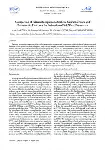
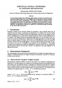
usually over-optimistic estimates of performance [Duda and Hart, 1973]. This is due to overspecialization of the classifier to the data.4 Techniques for estimating error rates have been widely studied in the statistics [Efron, 1982] and pattern recognition [Duda and Hart, 1973,Fukunaga, 1972] literature. The simplest technique for "honestly' estimating error rates, the holdout or H method, is a single train and test experiment. The sample cases are broken into two groups of cases: a training group and a test group. The classifier is independently derived from the training cases, and the error estimate is the performance of the classifier on the test cases. A single random partition of train and test cases can be somewhat misleading. The estimated size of the test sample needed for a 95%> confidence interval is described in [Highleyman, 1962]. With 1000 independent test cases, one can be virtually certain that the error rate on the test cases is very close to the true error rate. Instead of relying on a single train and test experiment, multiple random test and train experiments can be performed. For each random train and test partition, a new classifier is derived. The estimated error rate is the average of the error rates for classifiers derived for the independently and randomly generated partitions. Random resampling can produce better error estimates than a single train and test partition. A special case of resampling is known as leaving-one-out [Fukunaga, 1972, Efron, 1982]. LeavingOne-Out is an elegant and straightforward technique for estimating classifier error rates. Because it is computationally expensive, it is often reserved for relatively small samples. For a given method and sample size n, a classifier is generated using n-1 cases and tested on the remaining case. This is repeated n times, each time designing a classifier by leaving-one-out. Each case is used as a test case and, each time nearly all the cases are used to design a classifier. The error rate is the number of errors on the single test cases divided by n. Evidence for the superiority of the leaving-one-out approach is well-documented [Lachenbruch and Mickey, 1968, Efron, 1982]. While leaving-one-out is a preferred technique, with large samples it may be computationally expensive. However as the sample size grows, traditional train and test methods improve tneir accuracy in estimating error [Kanal and Chandrasekaran, 1971]. The leaving-one-out error technique is a special case of the general class of cross validation error estimation methods [Stone, 1974]. In k-fold cross validation, the cases are randomly divided into k mutually exclusive test partitions of approximately equal size. The cases not found in each test partition are independently used for training, and the resulting classifier is tested on the corresponding test partition. The average error rates over all k partitions is the cross-validated error rate. The CART procedure was extensively tested with varying numbers of partitions and 10-fold cross validation seemed to be adequate and accurate, particularly for large samples where leaving-one-out is computationally expensive IBreiman, Friedman, Olshen, and Stone, 1984]5 For small samples, bootstrapping, a method for resampling with replacement, has shown much promise as a low variance estimator for classifiers [Efron, 1983, Jain, Dubes, and Chen, 1987, Crawford, 1989]. This is an area of active research in applied statistics. Figure 1 compares the techniques of error estimation for a
4In the extreme, a classifier can be constructed that simply consists of all patterns in the given sample. Assuming identical patterns do not belong to different classes, this yields perfect classification on the sample cases. 5Empirical results also support the stratification of cases in the train and test sets to approximate the percentage (prevalence) of each class in the overall sample.
782
Machine Learning
sample of n cases. The estimated error rate is the average of the error rates over the number of iterations. While these error estimation techniques were known and published in the 1960s and early 1970s, the increase in computational speeds of computers, makes them much more viable today for larger samples and more complex classification techniques [Steen, 1988].
Figure 1: Comparison of Techniques for Estimating Error Rates
Besides improved error estimates, there are a number of significant advantages to resampling. The goal of separating a sample of cases into a training set and testing set is to help design a classifier with a minimum error rate. With a single train and test partition, too few cases in the training group can lead to the design of a poor classifier, while too few test cases can lead to erroneous error estimates. Leaving-OneOut, and to a lesser extent random resampling, allow for accurate estimates of error rates while training on most cases. For purposes of comparison of classifiers and methods, resampling provides an added advantage. Using the same data, researchers can readily duplicate analysis conditions and compare published error estimates with new results. Using only a single random train and test partition introduces the possibility of variability of partitions to explain the divergence from a published result. 2.2. Classification Methods In this section, the specific classification methods used in the comparison will be described. We do not review the methods or their mathematics, but rather state the conditions under which thev were applied. References to all methods are readily available. Our goal is to apply each of these methods to the same data sets and report the results. 2.2.1. Statistical Pattern Recognition Several classical pattern recognition methods were used. Figure 2 lists these methods. These methods are wellknown and will not be discussed in detail. The reader is referred to [Duda and Hart, 1973] for further details. Instead, we give the specific variation of the method that we used.
simplifies the normality assumption to equal covariance matrices. This is probably the most commonly used form of discriminant analysis; we used the canned SAS and IMSL programs. A recent report has demonstrated improved results in game playing evaluation functions using the quadratic classifier [Lee, 1988]. We used the nearest neighbor method (k=l) with the Euclidean distance metric. This is one of the simplest methods conceptually, and is commonly cited as a basis of comparison with other methods. It is often used in casebased reasoning [Waltz, 1986]. Bayes rule is the optimal presentation of minimum error classification. All classification methods can be viewed as approximations to Bayes optimal classifiers. Because the Bayes optimal classifier requires complete probability data for all dependencies in its invocation, tor real problems this would be impossible. As with other methods, simplifying assumptions are made. The usual simplification is to assume conditional independence of observations. While one can point to dozens of classifiers that have been built (particularly in medical applications [Szolovits and Pauker, 1978]) using Bayes rule with independence, such approaches have also been recently reported in the AI literature (although in the context of unsupervised learning) [Cheeseman, 1988]. Although independence is commonly assumed, there are mathematical expansions to incorporate higher order correlations among the observations. In our experiments, we tried both Bayes with independence and Bayes with the second order Bahadur expansion.6 2.2.2. Neural Nets A fully connected neural net with a single hidden layer was considered. The back propagation procedure [McClelland and Rumelhart, 1988] was employed and the general outline of the data analysis described in [Gorman, 1988] was followed. The specific implementation used was [McClelland and Rumelhart, 1988].7 In most experiments a learning rate of 1 and a momentum of 0 was used.8 Patterns were presented randomly to the learning system.9. The analysis model of [Gorman, 1988] corresponds to a 10-fold cross validation. Unlike the other methods examined in this study, back propagation usually commences with the network weights in a random state. Thus, even with sequential presentation of cases, the weights for one learned network are unlikely to match the same network that starts in a different random state. There is also the possibility of the procedure reaching a local maximum. In this analysis model, for each train and test experiment, the weights are learned 10 times, and test results averaged over all 10 experiments. Therefore, 10 times the usual number of training trials must be considered. For a 10-fold cross-validation, 100 learning experiments are made. For each data set, these experiments were repeated for networks having 0,2,3,6,9,12, or 24 hidden units (in a single layer). This is equivalent to using resampling to estimate the appropriate numoer of hidden units. Because the data sets may not be separable with these numbers of hidden units, we took the following measures to determine a sufficient
amount of computation time. Before doing the train and test experiments, the nets were trained several times on all samples for all size hidden units. We determined a number of epochs, i.e. complete presentations of the data set, that was sufficient to result in each increment of additional hidden units fitting the cases better than the lesser number of hidden units. In addition, for one problem where the data set was extremely large, we sampled the results every 500 epochs, and computed whether the average total squared error continued to be reduced. This indicated whether progress was being made. One output unit was used for each class. The hypothesis with the highest weight was selected as the conclusion of the classifier, and the error rate was computed. This is the general outline of the procedures followed. In Section 3, we describe the variations on this theme that were necessary for the specific data set analyses. For computational reasons, in some instances it was necessary to reduce the number of repeated trials to be averaged. For back propagation, we described a computational procedure that performed 10 train and test experiments for each one that would be necessary for other methods. However, the data sets described in Section 3 are not readily separable. Thus, the computation demands are quite large. We estimate that 6 months of Sun 4/280 cpu time were expended to compute the neural nets results in Section 3. 2.2.3. Machine Learning Methods In this category, we place methods that produce logistic solutions. As indicated earlier these methods have been explored by both the machine learning and statistics community. These are methods that produce solutions posed as production rules or decision trees. Conjunction or disjunction may be used as well as logical comparison operators on continuous variables such as greater than or less than. Predictive Value Maximization [Weiss, Galen, and Tadepalli, 1987] was tried on all data sets. This is a heuristic search procedure that attempts to find the best single rule in disjunctive normal form. It can be viewed as a heuristic approximation to exhaustive search. It is applicable to problems where a relatively short rule provides a good solution. For such problems, it should have an advantage in that many combinations are considered, in contrast to current decision tree procedures that split nodes without considering combinations. For more complex problems, a decision tree procedure is preferable. The appropriate rule length or tree size is determined by resampling. In addition, for two of the smaller data sets, an exhaustive search was performed for the optimal rule of length 2 in disjunctive normal form. For the other 2 data sets, the published decision tree results are available for methods using variations of ID3 and its successor C4.
3 Results In this section, we review the results of the various classification methods on four data sets. All of the data sets have been published, and in most instances we attempted to perform the analyses in a manner consistent with previously known results. 3.1. I r i s Data The iris data was used by Fisher in his derivation of the linear discriminant function [Fisher, 1936], and it still is the standard discriminant analysis example used in most current statistical routines such as SAS or IMSL. Linear or quadratic discriminants under assumptions of normality perform extremely well on this data set. Three classes of iris are discriminated using 4 continuous features. The data set consists of 150 cases, 50 for each class. Figure 3 summarizes the results. The first error rate is the apparent error rate on all cases; the second error rate is the leaving-
Weiss and Kapouleas
783
784
Machine Learning
3.3. Cancer Data A data set for evaluating the prognosis of breast cancer recurrence was analyzed by Michalski's AQ15 rule induction program and reported in [Michalski, Mozetic, Hong, and Lavrac, 1986]. They reported a 64% accuracy rate Tor expert physicians, and a 68% rate for AQ15, and a 72% rate tor the pruned tree procedure of ASSISTANT [Kononenko, Bratko, and Roskar, 1986], a descendant of ID3. 13 The authors derived the error rates by randomly resampling 4 times using a 70% train and a 30% test partition. Tne samples consist of 286 samples, 9 tests, and 2 classes. We created 4 randomly sampled data sets with 70% train and a 30% test partitions; each method was tried on each of the four data sets and the results averaged. Thus, the experimental results are consistent with the original study. Figure 7 summarizes the results. The first error rate is the apparent error rate on the training cases; the second error rate is the error rate on the test cases.
Figure 8: Neural Net Error Rates for Cancer Data
Figure 7: Comparative Performance on Cancer Data
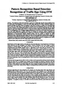
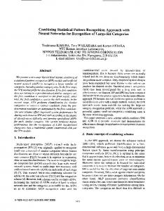
The rule-based solution has 1 rule with a total of 2 variables.14 For the neural nets, the apparent error rate is the average of ten training trials. Each testing result is the corresponding average testing result of tne same 10 complete trials.15 The nets were trained for 2000 epochs. The best neural net in terms of cross-validated error occurs at 0 hidden units, and is the one listed in Figure 7. The relationship between the number of hidden units and the error rates is listed in Figure 8. 3.4. T h y r o i d Data Quinlan reported on results of his analysis of hypothyroid data in [Quinlan, 1987b], and in greater detail in [Quinlan, 1987a]. The problem is to determine whether a patient referred to the clinic is hypothyroid, the most common thyroid problem. In contrast to the previous applications, relatively large numbers of samples are available. The samples consist of 3772 cases from the year 1985. These are the same cases used in the original report and were used for training. The 3428 cases from 1986 were used as test cases. There are 22 (principal) tests, and 3 classes. Over 10% of the values are missing because some lab tests were deemed unnecessary. For purposes of comparison of
the methods, these values were filled in with the mean value for the corresponding class. Figure 9 summarizes the results.16 The first error rate is the error rate on the 3772 training cases; the second error rate is the error rate on the 3428 test cases. From a medical perspective, it is known that (based on lab tests) excellent classification can be achieved for diagnosing thyroid dysfunction. For these data, the correct answer stored with each sample is derived from a large rule-based system in use in Australia. While most error rates in Figure 9 are low, it is important to note that 1% of the total sample represents over 70 people. Over 92% of the samples are not hypothyroid. Therefore, any acceptable classifier must do significantly better than 92%.
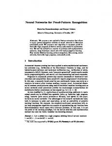
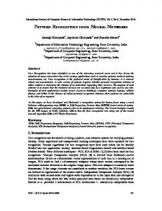
Figure 9: Comparative Performance on Thyroid Data The rule-based solution has 2 rules with a total of 8 variables. For the neural nets, the apparent error rate is the best of 2 trials. The nets were trained for 2000 epochs. The best neural net in terms of testing error occurs at 3 hidden units. The relationship between tne number of hidden units and the error rates is listed in Figure 10.
Weiss and Kapouleas
785
Figure 10: Neural Net Error Rates for Thyroid Data
The cpu times for training a neural net with back propagation on this size data set were great: for 3 hidden units 500 epochs required 1.5 hours of Sun 4/280 cpu time, while 24 units required 11.5 hours. In Figure 10, the apparent error rates for the larger numbers of hidden units support the hypothesis that additional training was necessary. We initiated a new set of experiments with fewer numbers of hidden units.17 We let these trials run for an unlimited period of time as long as slight progress was being made, as indicated by sampling every 500 epochs. Therefore, for this experiment not every size neural net was run an equal number of epochs. Figure 11 summarizes the results of this effort The best result encountered during the sampling of results occurred for 3 hidden units, and this result is listed in Figure 9.
Figure I I : Extended Neural Network Training on Thyroid Data
4 Discussion The applications presented here represent a reasonable cross section of prototypical problems widely encountered in the many research communities. Each problem has few classes and is characterized by uncertainty of classification. In some applications such as the cancer data, the features were relatively weak and good predictive capabilities are unlikely. In others, such as the thyroid data, the features are quite strong, and almost error-free prediction is possible. For the smaller data sets, resampling was used. With over 100 cases, resampling techniques such as cross-validation should give excellent estimates for the true error rate. In
The momentum was changed to .9, and the learning rate to .5. to help prevent local maximums.
786
M a c h i n e Learning
fact, the data from the iris study has been reviewed over many years, and comparisons have been made on the basis of the leaving-onc-out error. It is interesting to note (for those who wish to avoid concepts such multivariate distributions and covariance matrices), that a trivial set of 2 rules with a total of 3 variables can produce equal results. For many application fields, this in fact is a major advantage of the logistic approaches, i.e. the rule based or decision tree based approaches. The solution is compatible with elementary human reasoning and explanations. It is also compatible with rule-based systems. Thus, if everything were equal, many would choose the logistic solution. In our experiments, everything was not equal. In every case a logistic solution was found that exceeded the performance of solutions posed using different underlying models. PVM has an advantage when a short rule works, but for more complex problems the decision tree would be indicated. We note that the largest problem studied, the thyroid application, is somewhat biased towards logistic solutions. The endpoints were derived from a rule-based system that apparently uses the same lab test thresholds to specify high or low readings for all hypotheses. These results cannot necessarily be extrapolated to more complex problems. However, our experience is not unique. Numerous experiments by the developers of CART [Breiman, Friedman, Olshen, and Stone, 1984] demonstrated that in most instances, they found a tree superior to alternative statistical classification techniques. In our experiments, the statistical classifiers performed consistently with expectations. The linear classifiers (with the assumption of a normal distribution) gave good performance in all cases except the thyroid experiment. These classifiers are widely used, because they are simple and the training error rate usually holds up well on lest cases. The natural extension, the quadratic classifier, fits better to normally distributed data, but degrades rapidly with nonnormal data. It did poorly in most of our experiments. Similarly Bayes with independence does moderately well, but the 2nd order fits were not good on the test data. Nearest neighbor does well with good features, but tends to degrade with many poor features. There are many alternative statistical classifiers that might be tried, such nonparametric piecewise linear classifiers [Foroutan and Sklansky, 1985]. In addition, one could try to reduce the number of features for training (i.e. feature selection), since many of these methods can actually improve performance on test cases by feature reduction.18 The neural nets did perform well, and they were the only statistical classifiers to do well on the thyroid problem. However, overall they were not the best classifiers; they consumed enormous amounts of cpu time; and they were sometimes equaled by simple classifiers. Research on improving performance for neural nets training and representation is quite active, so it may be possible that performance can be improved. The relationship between the number of hidden units and the two error rates followed the classical pattern for classifiers. As the number of hidden units increased, the apparent error decreased.19 However, at some point, as the classifier overfits the data, the true error rate curve flattens and even begins to increase. Much the same behavior can be observed for decision trees as the number of nodes increases, or production rules, as the rule length increases.
18 Because the linear classifier performed poorly on the thyroid cases, we tried to train a classifier on just the lab tests, which are the most significant tests. The results did not improve. 19 Occasionally there is some slight variability in the decrease of the apparent error rate because back propagation minimizes distance as opposed to errors.
The question remains open as to how well any classifier can do on more complex problems with many more features and many more classes, possibly non-mutually exclusive classes. There are also questions of how many cases are actually needed to learn significant concepts. Our study does not answer many of these questions, but helps show in a limited fashion where we are currently with many commonly used classification techniques.
Appendix: Induced Rules • iris. Petal length < 3 -> Iris Setosa; Petal length > 4.9 OR Petal Width > 1.6-> Iris Virginica • appendicitis. MNEA>6600 OR MBAP>11 • cancer. Involved Nodes>0 & Degree=3 • thyroid. TSH>6.1 & F T I primary hypothyroid; TSH>6 & TT464 & Surgery=false -> compensated hypothyroid
References
Chen, C. Bootstrap Techniques for Error Estimation. IEEE Transactions on Pattern Analysis and Machine Intelligence. 9(1987)628-633. [James, 1985] James, M. Classification Algorithms. York: John Wiley & Sons, 1985.
New
[Kanal and Chandrasekaran, 1971] Kanal, L. and Chandrasekaran On Dimensionality and Sample Size In Statistical Pattern Classification. Pattern Recognition. (1971)225-234. [Kononenko, Bratko, and Roskar, 1986] Kononcnko, I., Bratko, I., Roskar, E. ASSISTANT: A System for Inductive Learning. Informatica. 10 (1986). [Lachenbruch and Mickey, 1968] Lachenbruch, P. and Mickey, M. Estimation of Error Rates in Discriminant Analysis. Technometrics. (1968) 1-111. [Lee, 1988] Lee K. and Mahajan S. A Pattern Classification Approach to Evaluation Function Learning. Artificial Intelligence. 36(1988) 1-25.
[Baum, 1989] Baum E. What Size Net Gives Valid Generalization? Neural Computation. (1989).
[Marchand, Van Lente, and Galen, 1983] Marchand, A., Van Lente, F., and Galen, R. The Assessment of Laboratory Tests in the Diagnosis of Acute Appendicitis. American Journal of Clinical Pathology. 80:3 (1983) 369-374.
[Breiman, Friedman, Olshen, and Stone, 1984] Breiman, L., Friedman, J., Olshen, R., and Stone, C. Classification and Regression Tress. Monterrey, Ca.: Wadsworth, 1984.
[McClelland and Rumelhart, 1988] McClelland, J. and Rumelhart, D. Explorations in Parallel Distributed Processing. Cambridge, Ma.: M I T Press, 1988.
[Cheeseman, 1988] Cheeseman P., Self M., Kelly J., Stutz J., Taylor W., and Freeman D. Bayesian Classification. In Proceedings of AAAI-88. Minneapolis, 1988,607-611.
[Michalski, Mozetic, Hong, and Lavrac, 1986] Michalski, R., Mozetic, I., Hong, J., and Lavrac, N. The Multi-purpose Incremental Learning System AQ15 and its Testing Application to Three Medical Domains. In Proceedings of the Fifth Annual National Conference on Artificial Intelligence. Philadelphia, Pa., 1986, 1041-1045.
[Clancey, 1985] Clancey, W. Heuristic Classification. Artificial Intelligence. 27 (1985) 289-350. [Crawford, 1989] Crawford, S. Extensions to the C A R T Algorithm. International Journal of Man-Machine Studies. (1989) in press. [Duda and Hart, 1973] Duda, R., and Hart, P. Pattern Classification and Scene Analysis. New York: Wiley, 1973. [Efron, 1982] Efron, B. The Jackknife, the Bootstrap and Other Resampling Plans. In S I A M . Philadelphia, Pa., 1982. [Efron, 1983] Efron, B. Estimating the Error Rate of a Prediction Rule. Journal of the American Statistical Association. 78 (1983) 316-333.
[Quinlan, 1986] Quinlan, J. Induction of Decision Trees. Machine Learning. 1 (1986) 1. [Quinlan, 1987a] Quinlan, J. Simplifying Decision Trees. International Journal of Man-Machine Studies. (1987) 221-234. [Quinlan, Rules from International Milan, Italy,
1987b] Quinlan, J. Generating Production Decision Trees. In Proceedings of the Tenth Joint Conference on Artificial Intelligence. 1987, 304-307.
[Steen, 1988] Steen, L. The Science of Patterns. Science. 240(1988)611-616.
[Fisher, 1936] Fisher, R. The Use of Multiple Measurements in Taxonomic Problems. Ann. Eugenics. 1 (1936) 179-188.
[Stone, 1974] Stone, M. Cross-Validatory Choice and Assessment of Statistical Predictions. Journal of the Royal Statistical Society. 36(1974) 111-147.
[Foroutan and Sklansky, 1985] Foroutan, I. and Sklanskv, J. Feature Selection for Piecewise Linear Classifiers. In IEEE Proc. on Computer Vision and Pattern Recognition. San Franscisco, 1983,149-154.
[Szolovits and Pauker, 1978] Szolovits, P., and Pauker, S. Categorical and Probabilistic Reasoning in Medical Diagnosis. Artificial Intelligence. 11 (1978) 115-144.
[Fukunaga, 1972] Fukunaga, K. Introduction to Statistical Pattern Recognition. New York: Academic Press, 1972. [Gorman, 1988] Gorman R. and Seinowski T. Analysis of Hidden Units in a Layered Network Trained to Classify Sonar Targets. Neural Networks. 1 (1988)75-89. [Haussler, 1988] Haussler, D. Quantifying Inductive Bias: AI Learning Algorithms and Valiant s Learning Framework. Artificial Intelligence. 36(1988)177-221. [Highleyman, 1962] Highleyman, W. The Design and Analysis of Pattern Recognition Experiments. Bell System Technical Journal. 41 (1962) 723-744. [Jain, Dubes, and Chen, 1987] Jain, A., Dubes, R., and
[Valiant, 1985] Valiant, L.G. Learning disjunctions of conjunctions. In Proceedings of IJCAI-85. Los Angeles, 1985, 560-566. [Waltz, 1986] Stanfill G. and Waltz D. Toward MemoryBased Reasoning. Communications of the ACM. 29 (1986) 1213-1228. [Weiss and Kulikowski, 1984] Weiss, S. and Kulikowski, C. A Practical Guide to Designing Expert Systems. Totowa, New Jersey: Rowman and Ailanheld, 1984. [Weiss, Galen, and Tadepalli, 1987] Weiss, S., Galen, R., and Tadepalli, P. Optimizing the Predictive Value of Diagnostic Decision Rules. In Proceedings of the Sixth Annual National Conference on Artificial Intelligence. Seattle, Washington, 1987,521-526.
Weiss and Kapouleas
787