An Inter-arrival Delay Jitter Model using Multi-Structure. Network Delay Characteristics for Packet Networks. EdwardJ Daniel, Christopher M White, and Keith A.
An Inter-arrival Delay Jitter Model using Multi-Structure Network Delay Characteristics for Packet Networks EdwardJ Daniel, Christopher M White, and Keith A. Teague School of Electrical and Computer Engineering Oklahoma State University Stillwater, OK buffering to overcome this problem can lead to excessive end to end delay in the system.
ABSTRACT Data traversing packet networks experience varying delays, resulting in inter-arrival jitter. This can result in degraded performance in real-time multimedia communications applications if the jitter delays are large or unaccounted for in the receiver application. This paper examines modeling and simulation of network jitter delay for real-time multimedia communications applications. We examine the multi-structure characteristics of network delay and develop a model for simulation of jiqer. T h e model is c o n f m e d empirically using collected packet network jitter delay statistics.
In this paper, we examine the characteristics of network delay jitter to develop a model for network interamval jitter. Section 2 describes the characteristics of packet network inter-arrival delay. Section 3 presents our network delay jitter model. Section 4 gives comparisons of ow model to empirically collected network jitter data. Finally, in Section 5 summary and conclusions are given.
2. NETWORK JITTER DELAY PROPERTIES
.~
..
.,:
..
I..:INTRODUCTION . . .
When a real-time voice communication application
.
Packet-switched networks are being used to provide interactive muliimedia communications, including realtime voice, video and data services. However, packet networks are','. not ideal for real-time multimedia app1ications":'such' as voice communications. Packet networks exhibit non-ideal behavior that may seriously degrade the performance of real-time communications systems. Particularly, as packets are transmitted from source to .destination, they may experience different delays. As a result, packets arrive at the destination with varying delays (between packets) referred to as 'jitter'. Packet delay jitter may result from packets taking different paths to their destination to avoid congested areas or failed links. However, jitter is primarily caused by varying queuing delays encountered by packets at routers (nodes). Network packets compete with other networks traffic at routers. Routers statistically multiplex incoming packets, which results in the varying delay. .
.
In a voice over IP (VoIF') application, large interarrival jitter leads to starvation of the audio playback system. If there is not adequate buffering on the received system these delays will lead to packet loss and a corresponding loss of voice data (seen at playback). Data
0-7803-8104-1/03/$17.00 02003 IEEE
1738
uses a wide area packet network employing IP (Internet Protocol) to transmit a stream of voice data, referred to as a tagged stream, it is multiplexed at network nodes (routers) with the other traffic on the network called background traffic. IP network nodes have no priorities, so network traffic is serviced on a First in First out (FIFO) basis. Therefore, queuing delays and jitter experienced by packets are a direct result of wait and service times in the queue. Jitter delays of tagged streams on packet networks are a sample of the queuing delays of the background traffic at the nodes [ I ] [2]. The relative size of the tagged stream is small compared to the background traffic, so it does not significantly contribute to the queuing delays. As tagged stream packets travel across a network path they sample the busy periods' (and queuing delays) of the nodes along the path [3]. If the send rate, or the time between packets, of the tagged stream is smaller than the busy periods of the node, the tagged stream gets a sample of the queuing delays within the busy periods (more than one sample from the same busy period), Figure I(a). However, when the send rate is larger than the busy
'
When several packets anive at the node during a given interval (possibly simultaneously), it is referred to as a busy period.
..
periods, the tagged stream samples delays of different busy periods (many different busy periods), Figure I(b). Essentially, larger send rates sample the busy periods while smaller send rates sample the delays within the busy periods.
characteristic to its large time scale characteristic is referred to as the crossover. Several researchers have developed complex models and performed empirical simulation studies of network jitter including [I] [2] [5]. These studies show that network jitter follows a Laplacian distribution. Yletyinen and Kantola ([SI) showed that the probability distribution function widens and shortens based on increases in traffic load, utilization, burstiness, and burst length. Widening of the Laplacian pdf signifies higher probabilities of long jitter delays, while shortening of the pdf implies higher probability for small jitter delays.
Interval between sampling of delys within bury periods
WRY
(0)
While investigating an adaptive jitter buffering algorithm, Ramjee el al. [6] reported the delay spike phenomena, a condition where a delay spike in a packet stream is proceeded by a series of packets arriving very close together. When a packet experiences a large delay, the packets following get “held up” and as a result they all amve with very small inter-arrival times, sometimes almost simultaneously. Ramjee et ai. found that the delay spike phenomena decayed exponentially, and incorporated an exponential decaying function into the spike detection jitter buffering algorithm. When his jitter buffering algorithm detected a delay spike it was allowed to decay exponentially to follow the slope of the spike until it leveled off at approximately zero slope, signaling the end of the delay spike. This obviously indicates a correlation attribute of inter-arrival jitter delays.
InferVal between sampling of delays of busy peiods
I
Figure I . (a) Tagged stream sampling of queuing delay within busy periods and @) Tagged stream sampling of busy periods of a queue. W(t) is an instance of a queuing delay process and tgp represents the start time of a busy period. [3] According to Li and Mills [3], this sampling describes the multi-structure of delay, which consist of a short term non-stationary component, the delays within busy periods, and a long-term stationary component, the delays of different busy periods. The long-term stationary component can be modeled as a Gaussian noise process because there is no correlation between the occurrences of busy periods of a queue. Moreover, the delays sampled withiin the queue for each busy period have no correlation with delays sampled from other busy periods. The multistructure characteristic of network delay is used in the next section to develop a model for jitter.
3. NETWORK JITTER DELAY MODEL Li and Mills’ ([4]) study and analysis of network delay states that smaller sampling intervals can be modeled as a non-stationary process, while the longer time intervals can be modeled as a stationary process. The point at which the delay changes i?om its small time scale
1739
In our proposed jitter model, delays are generated i?om probability distributions that have no correlation between samples, thus not simulating delay spike characteristics. Therefore, an exponential decaying function is used to simulate this phenomenon when the Laplacian or Gaussian distribution produces a delay spike. The Laplacian distribution is used to model the small time scale, non-stationary, process, and the large time scale stationary process is modeled with additive Gaussian white noise. Jitter delay spikes and subsequentjitter delays follow the delay spike adjustment procedure noted above. The combination of the Laplacian distribution, Gaussian white noise, and delay spike adjustment provide a means to model the multi-structure characteristics of packet delay. The proposed model is shown in figure 2.
Additive Gaussian
Laplacian
Small time,
Large time scale delays
scale delays
Figure 3 shows the Laplacian distribution function implementation simulating 10,000 packets with a = 49 a n d P = 5 ,
Exponential Decaying
Delays following delay spikes
Figure 2. Proposed Jitter Model The Laplacim distribution is used to generate packet jitter delay values based on a specified mean and variance. The characteristic equations (I) and (2) for the Laplacian distribution function are given as follows:
Gaussian white noise is added to the delay values generated by the Laplacian distribution function to introduce the large time scale properties. This is done based on a sampling that follows the crossover value. For example, delay values are altered by the Gaussian white noise process at intervals based on the crossover from small time scale to large time scale. This process models sampling of the busy periods of the queue. When a delay spike is detected, based on a threshold, delay values following the delay spike are reduced exponentially, allowing them to “catch up” with the delayed (spike) packet. Equation (3) gives the exponential decay function used to model this characteristic. The number of proceeding packets that are affected by the delay spike is denoted as the spike i n f e n d In order for the packets following the spike to “catch up” with the delay spike the average jitter delays within a spike interval should he less than or equal to the mean.
a(()= d(f)e?‘, where,
a=meun and ,L3=
(3)
where, d#J is the inter-anival jitter at time 1. Figure 4 provides a pictorial description of this delay jitter adjustment process.
d‘;“
i
.
.
@0*11mI
Figure 4. Jitter delay spike adjustment procedure. (a) delay spike produced from model and (b) reduction of delays following delay spike.
Figure 3. Generated Laplacian Distribution using Laplacian Random Number Generator.
1740
4. JITTER MODEL COMPARISONS
6. The delay distributions follow a Laplacian distribution about the mean of 45ms.
Experiments were conducted with a Network Performance Application (Netpeg) that was specifically developed to collect packet network statistics for VoIP data. NetPeflis written in Visual C+k to operate under the MS Windows operating systems. The program runs as a serverlclient pair between two computers connected to an IP network (possibly concatenated networks). The application was specifically designed to send simulated voice compressed data over IP networks, with the flexibility to accommodate various user-specified data sizes and send rates, including IP packet parameters to simulate VoIP traffic such as frame sizes, packet size (or kames per packet), send rate, duration of simulation, etc. During a simulation Netperf appends packet sequence numbers on all outgoing packets, and records all packet send and amval times (keeping track of received packet numbers). This information is used to calculate packet statistical information, such as packet inter-arrival time (jitter), end-to-end packet delay, packet loss rate, etc. Accurate timing is critical for this application; therefore the two computer's (client and server) clocks must be carefully synchronized using Network Time Protocol (NTP) [7]. Netperf is a multithreaded architecture that uses multiple TCP connections for control and a UDP connection for data transfer. NefPefl was used to collect network inter-arrival delays between a PC connected to the Wide Area Internet via an office LAN (Local Area Network) and a remote PC connected to the Internet. The packet trace (stream of voice data) sent simulated voice data every 45ms,at 14 bytes of payload per packet, from server to client. The resulting inter-arrival delay jitter is compared with the data simulated from the network delay jitter model. The model was used to generate jitter delay values based on the statistical data reported by the Netper/ simulation. The jitter data collected empirically using NefPeflhad a mean of 45 ms and a standard deviation of 5.59. These values were used in determining the jitter model inputs to yield comparable results. A crossover of 180 ms, and a spike scale of 3 times the mean delay was used for Gaussian noise sampling and spike detection adjustment, respectfully. Figure 5 compares the collected jitter delays from Netperf and the jitter delays produced by the proposed multi-structure jitter model. The model returned a mean jitter of 45 ms with a standard deviation of 5.5, values equaling the NetPefldata.
Figure 5 shows that both the measured and modeled jitter are bursty, with the majority of the jitter delays appearing near the mean as expected. This is also evident in the inter-arrival delay jitter distribution shown in Figure
3000
4000
Packet Nwmber
o O ~ l O O O
2000
3000 4000 Packet Number
'
5000
____
5000
6000
6000
Figure 5. Measured vs. Model Jitter Delays
1 09,
Figure 6. Jitter Delay Dislribution for Measured and Modeled Jitter Delays. The data generated from the above simulation and jitter model was compared with trace data runs over LAN (connected to the Wide Area Internet) to a CDMA data network connection. Trace m s for several times of day were compared for the LAN to CDMA data trace to get a representation of different levels of busy periods. Normalized variance characteristics are compared by averaging variance values of m-aggregated time series. This technique is typically used for self-similarity determination, as illustrated in [XI. The m-aggregated time series x(*) = {$,k = OJ,Z ,...} ,of a stationary time series x, can be defmed by summing the original time series over
1741
non-overlapping, adjacent blocks of size m. The aggregated variance calculations essentially compress the time scales, with m=l representing the bighest magnification and m=10 a factor of I O reduction in magnification. This can be expressed as,
In this comparison an m-aggregate time series of the variance of the jitter delays is used, illustrated in equation (5)
v*r(p,= !‘o&,