An Object-Oriented Representation for Efficient Reinforcement Learning

An Object-Oriented Representation for Efficient Reinforcement Learning

Carlos Diuk CDIUK @ CS . RUTGERS . EDU Andre Cohen ACOHEN @ CS . RUTGERS . EDU Michael L. Littman MLITTMAN @ CS . RUTGERS . EDU RL3 Laboratory, Department of Computer Science, Rutgers University, Piscataway, NJ USA

Abstract Rich representations in reinforcement learning have been studied for the purpose of enabling generalization and making learning feasible in large state spaces. We introduce Object-Oriented MDPs (OO-MDPs), a representation based on objects and their interactions, which is a natural way of modeling environments and offers important generalization opportunities. We introduce a learning algorithm for deterministic OO-MDPs and prove a polynomial bound on its sample complexity. We illustrate the performance gains of our representation and algorithm in the wellknown Taxi domain, plus a real-life videogame.

1. Introduction In the standard Markov Decision Process (MDP) formalization of the reinforcement-learning (RL) problem (Sutton & Barto, 1998), a decision maker interacts with an environment consisting of finite state and action spaces. Algorithms for RL in MDP environments suffer from what is known as the curse of dimensionality: an exponential explosion in the total number of states as a function of the number of state variables. Learning in environments with extremely large state spaces is challenging if not infeasible without some form of generalization. Exploiting the underlying structure of a problem can enable generalization and has long been recognized as important in representing sequential decision tasks (Boutilier et al., 1999). In this paper, we propose an extension to the standard MDP formalism, which we call Object-Oriented MDPs (OOMDPs), and present an efficient learning algorithm for deterministic OO-MDPs. We claim that this object-based approach is a natural way of viewing and describing many real-life domains that enables multiple opportunities for Appearing in Proceedings of the 25 th International Conference on Machine Learning, Helsinki, Finland, 2008. Copyright 2008 by the author(s)/owner(s).

generalization. There are many ways of incorporating objects into models for learning and decision making—this paper explores one particular approach as a first attempt to understand the issues that arise. Our representation has multiple connections with other formalisms proposed in the Relational Reinforcement Learning literature (van Otterlo, 2005), but emphasizes simplicity and tractability over expressive power. Our representation starts from attributes that can be directly perceived by the agent, rather than predicates or propositions introduced by the designer (although we allow the encoding of prior knowledge in propositional form). A similar formalism, relational MDPs (RMDPs), was introduced by Guestrin et al. (2003) in the context of planning, and is based on the same insight. While our formalism has similarities to RMDPs, we introduce a number of changes, mainly in the way transition dynamics are described, to enable efficient learning and generalization. To present and test our approach, we first provide benchmark experiments in the well-known Taxi domain (Dietterich, 2000). We further demonstrate its applicability by designing an agent that can solve an interesting problem in the real-life videogame Pitfall1 .

2. Notation We use a standard Markov Decision Process (MDP) notation throughout this paper (Puterman, 1994). A finite MDP M is a five tuple S, A, T, R, γ. We use T (s |s, a) to denote the transition probability of state s given state– action pair (s, a) and R(s, a) to denote the expected reward value. A deterministic MDP is one in which there is a single next state s for every given state s and action a; that is, ∀s ∈ S, a ∈ A, ∃s ∈ S : T (s |s, a) = 1.

3. Object-oriented Representation We will use the Taxi domain, defined by Dietterich (2000), as an example to introduce our formalism. Taxi is a grid1

c 1982 Activision, Inc.


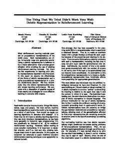
OO-MDP representation. Whereas in the classical MDP model, the effect of encountering walls is felt as a property of specific locations in the grid, the OO-MDP view is that wall interactions are the same regardless of their location. As such, agents’ experience can transfer gracefully throughout the state space.

Figure 1. The taxi domain. (a) Original 5 × 5 Taxi problem. (b) Extended 10 × 10 version, with a different wall distribution and 8 possible passenger locations and destinations.

world domain (see Figure 1.a), where a taxi has the task of picking up a passenger in one of a pre-designated set of locations (identified in the figure by the letters Y, G, R, B) and dropping it off at a goal destination, also one of the pre-designed locations. The set of actions for the taxi are North, South, East, West, PICKUP and DROPOFF. Walls in the grid limit the taxi’s movements. A common factored-state representation for the Taxi problem uses Dynamic Bayesian Networks (DBNs) to indicate how state variables influence each other. For example, the location of the taxi after a North action only depends on its current location and is independent of the passenger or destination variables. We depart from this representation and introduce one based on objects and their interactions. Many elements in our representation are similar to those of relational MDPs (Guestrin et al., 2003) with significant differences in the way we represent transition dynamics. Similar to RMDPs, we define a set of classes C = {C1 , . . . , Cc }. Each class includes a set of attributes Att(C) = {C.a1 , . . . , C.aa }, and each attribute has a domain Dom(C.a). A particular environment will consist of a set of objects O = {o1 , . . . , oo }, where each object is an instance of one class: o ∈ Ci . The state of an object o.state is a value assignment to all its attributes. The state of the underlying o MDP is the union of the states of all its objects: s = i=1 oi .state. An OO-MDP representation of Taxi has four object classes: Taxi, Passenger, Destination and Wall. Taxi, Passenger and Destination have attributes x and y, which define their location in the grid. Passenger also has a Boolean attribute in-taxi, which specifies whether the passenger is inside the taxi. Walls have an attribute that indicates their position in the grid. The Taxi domain, in its 5 × 5 version shown in Figure 1.a, has one object of each class Taxi, Passenger, and Destination, and multiple (26) objects of class Wall. This list of objects points out a significant feature of the

When two objects interact in some way, they define a relation between them. A combination of the relation established, plus the internal states of the two objects, determines an effect—a change in value of one or multiple attributes in either or both interacting objects. This behavior is defined at the class level, meaning that different objects that are instances of the same class behave in the same way when interacting with other objects. Formally, a relation r : Ci × Cj → Boolean is a function, defined at the class level, over the combined attributes of objects of classes Ci and Cj . Its value gets defined when instantiated by two objects o1 ∈ Ci and o2 ∈ Cj . For our Taxi representation, we will define 5 relations: touchN (o1 , o2 ), touchS (o1 , o2 ), touchE (o1 , o2 ), touchW (o1 , o2 ) and on(o1 , o2 ), which define whether an object o2 ∈ Cj is exactly one cell North, South, East or West of an object o1 ∈ Ci , or if both objects are overlapping (same x, y coordinates). Different domains require different relations. When the object taxii ∈ Taxi is on the northern edge of the grid and tries to perform a North action, it hits some object wallj ∈ Wall and the observed behavior is that it doesn’t move. We say that a touchN (taxii , wallj ) relation has been established and the effect of an action North under that condition is no-change. On the other hand, if ¬touchN (taxii , wallj ) is true and the taxi performs the action North, the effect will be taxii .y ← taxii .y + 1. As stated before, these behaviors are defined at the class level, so we can refer in general to the relation touchN (Taxi, Wall) as producing the same kind of effects on any instance of taxii ∈ Taxi and wallj ∈ Wall. We define some properties of these transition dynamics more formally in the next section. 3.1. Transition Dynamics Every state s induces a certain value assignment to all attributes of all objects—and therefore all relations—in the domain. Transitions are determined by interactions between objects. Every pair of objects o1 ∈ Ci and o2 ∈ Cj , their internal states o1 .state and o2 .state, an action a, and the set of relations r(o1 , o2 ) that are true—or false—at the current state, determine an effect—a change of value in some of the objects’ attributes. Definition 1 An effect is a single operation over a single attribute att in the OO-MDP. We will group effects into types, based on the kind of operation they perform. Ex-


amples of types are arithmetic (increment att by 1, subtract 2 from att), and constant assignment (set att to 0). Definition 2 A term t is any Boolean function. In our OOMDP representation, we will consider terms representing either a relation between two objects, a certain possible value of an attribute of any of the objects or, more generally, any Boolean function defined over the state space that encodes prior knowledge. All transition dynamics in an OO-MDP are determined by the different possible settings of a special set of terms called T . Definition 3 A condition is a set Tc of terms and negations of terms from T that must be true in order to produce a particular effect e under a given action a. We can summarize an OO-MDP transition cycle as follows:

1: while agent is acting do 2: Agent observes current state s and returns action a. 3: From state s, the environment extracts all relations

4:

5: 6: 7: 8: 9:

that currently hold between objects and observes the value of all attributes of all objects, assigning a True/False value to all terms in T . For each (if any) fulfilled condition in Tc , there’s an effect that will occur, determining a set of effects to be applied to s. If no conditions were fulfilled, no change takes place to s. Otherwise, the environment uses the set of effects to compute s . New state s ← s . The environment chooses a reward r from R(s, a). Agent is told r. end while

4. DOORMAX: Learning and Solving Deterministic OO-MDPs We introduce Deterministic Object-Oriented Rmax (DOORMAX), an algorithm for learning and solving deterministic OO-MDPs. DOORMAX is correct and, as we will show, provably efficient under the following assumptions. Assumption 1 For each action and each attribute, only effects of one type can occur. Assumption 2 For every action a, attribute att and effect type t, there is a set CE of condition–effect pairs that determine changes to att given a. No effect can appear twice on this list, and there are at most k different pairs—|CE| ≤ k. Plus, no conditions Ti and Tj in the set CE contain each

other: ¬(Ti ⊂ Tj ∨ Tj ⊂ Ti ). The number of terms or negations of terms in any condition is bounded by a known constant M . Assumption 3 Effects are invertible, that is, given states s and s , for each attribute att and each effect type we can determine a unique effect that would transform att from its value in s to its value in s . 4.1. Definitions and Data Structures We introduce some definitions, notation, and data structures that will be used to describe DOORMAX: • T is the union of all terms t that will be involved in the conditions that determine the transition dynamics of the environment described by the OO-MDP, plus their negations ¬t, with |T | = 2n. • For every state s ∈ S, the function cond(s) returns the subset of terms in T that are true in s. • A condition Tc ⊆ T is represented by a string cS of length n, where ciS = 1 if ti ∈ Tc , ciS = 0 if ¬ti ∈ Tc and ciS = * if ti ∈ / Tc ∧ ¬ti ∈ / Tc . • Given two conditions represented as strings c1 and c2 , we define the commutative operator ⊕ : c × c → c as follows: c1 c2 c1 ⊕ c2 0 0 0 1 1 1 1 * 0 * 0|1 * • A condition c1 matches another condition c2 , noted c1 |= c2 , if ∀1 ≤ i ≤ n : ci1 = * ∨ ci1 = ci2 . • For any states s and s and attribute att, the function effatt (s, s ) returns one effect of each type that would transform attribute att in s into its value in s . • A prediction p is a pair (p.model, p.effect), where p.model is a condition that represents the set of terms that need to be true for p.effect to occur. • For each action a, each attribute att and each effect type type, a set of predictions pred(a, att, type) is maintained. We refer to the set of models in a set of predictions as pred(a, att, type).models. • If an action a produces no effect from a given state s (s = s), we call the induced condition cond(s) a failure condition. We define Fa to be a set of failure conditions for action a. • Two effects are incompatible if, for any initial value of an attribute, applying these two effects would yield two different final values.


4.2. OO-MDP Representation of Taxi To facilitate understanding of the notation and data structures, we present a full example of our representation in the Taxi domain.

Whenever we observe a new condition ci such that any existing condition in FNorth matches it, we predict that performing a North action will have no effect. 4.3. Learning Algorithm

The set of terms T , which determines the transition dynamics of the OO-MDP, includes the four touchN/S/E/W relations between the taxi and the walls; the relevant relations between the taxi and the passenger and destination; the attribute value passenger.in-taxi = T ; and all their negations:

The DOORMAX algorithm (Algorithm 1) follows the general structure of most RL algorithms in the Rmax family, which work as follows. Using examples of transitions (s, a, s ), a learning algorithm constructs the transition model T . The learning algorithm must satisfy the KWIK (knows what it knows) conditions (Li et al., 2008), on(taxi, passenger), { touchN/S/E/W (taxi, wall), which say: (1) all predictions must be accurate (assuming a ¬touchN/S/E/W (taxi, wall), ¬on(taxi, passenger), valid hypothesis class), and (2) however, the learning algoon(taxi, destination), ¬on(taxi, destination), rithm may also return ⊥, which indicates that it cannot yet passenger.in-taxi = T , passenger.in-taxi = F } predict the output for this input. The sample complexity or KWIK bound of a learning algorithm is the maximum Consider the state s where the taxi is in position (2, 4) (as number of times it returns ⊥. In the Rmax setting, any in Figure 1.a), the passenger is inside the taxi, and the destransition that cannot yet be predicted is assumed to lead to tination is G. For this state, the function cond(s) returns: a fictious smax state from which maximum reward can be ¬touchS (taxi, wall), { touchN (taxi, wall), obtained. touchW (taxi, wall), ¬touchE (taxi, wall), ¬on(taxi, passenger), ¬on(taxi, destination), Algorithm 1 DOORMAX: main() method passenger.in-taxi = T }. 1: // Set up data structures: 2: for all actions a ∈ A do The corresponding 7-character string representation for this 3: Fa ← ∅ condition is 1001001, following the prior order for the 4: for all attributes att ∈ c∈C Att(c) do terms. 5: for all effect types type do Let’s now assume that the agent tries to perform the ac6: pred(a, att, type) ← ∅ tion East, which takes it to state s where the taxi is in 7: Add pred(a, att, type) to set of active prediclocation (3, 4). The corresponding cond(s ) is similar, extions P cept that now the taxi is not touching a wall to its West 8: end for (¬touchW (taxi, wall)). The corresponding string represen9: end for tation of the new condition is: 1000001. The observed ef10: end for fect is that the taxi moved to location (3, 4). In our repre11: while ¬(Termination criterion) do sentation, two effect types are allowed: arithmetic and con12: Observe current state s. stant assignment. Therefore, the function efftaxi.x (s, s ) 13: Choose action a according to exploration polwill return two values: increment(1) and set-to(3). icy, based on prediction for T (s |s, a) returned by predictTransition(s, a). Now, the agent takes another East action, and gets to state 14: Observe new state s . s , where location is (4, 4), it’s touching a wall to the East 15: Update learned model using method and standing on the destination. cond(s ) can now be rep addExperience(s, a, s , k). resented as 1010011. The two observed effects to taxi.x are 16: end while increment(1) and set-to(4). Note that the transition model for an OO-MDP need not predict the changes to the conditions, only to the attributes. The condition values are then derived separately using the knowledge of the relevant relations and their definitions. Finally, we’ll consider separately the actions that produce no effect. Let’s assume the agent also attempted an action North from each of the previous states, which resulted in it hitting a wall and staying in the same state. We treat these cases differently: The corresponding conditions 1001001, 1000001 and 1010011 will be identified as failure conditions for action North and incorporated into the set FNorth .

The two main routines of the algorithm are predictTransition (Algorithm 2), which predicts the next state given a current state and action based on the current model, and addExperience (Algorithm 3), which learns a model of the OO-MDP. If predictTransition is not able to predict a next state with accuracy, it returns smax . To help understand these routines, we present a couple of intuitions, based on the Taxi examples presented in the previous section. Notice that if we applied the ⊕ operator to


cond(s) and cond(s ), the two conditions from which an East action produced an increment(1) effect, we would obtain: 1001001 ⊕ 1000001 = 100*001. The resulting condition indicates that the term touchW (wall, taxi) is irrelevant with respect to action East and effect increment(1). If we also compare the two pairs of effects obtained, we observe that we consistently observed increment(1), whereas set-to(3) and set-to(4) are incompatible effects. These observations constitute the central ideas for the learning algorithm. Algorithm 2 predictTransition(s,a) method 0: Inputs: state s and action a. 0: Output: a predicted state s ∈ S ∪ {smax }. 1: if ∃c ∈ Fa s.t. c |= cond(s) then 2: // The current condition is a known failure condition. 3: Return s 4: else 5: for all attributes att ∈ c∈C Att(c) do 6: E←∅ 7: for all effect types type do 8: if ∃p ∈ pred(a, att, type) s.t. p.model |= cond(s)S then 9: Add p.effect to E 10: end if 11: end for 12: if E = ∅ ∨ ∃ei , ej ∈ E s.t. ei and ej are incompatible then 13: Return smax 14: else 15: // Set E contains all the individual operations that need to be applied to attributes in s in order to convert it to s . 16: s ← apply E to s 17: Return s 18: end if 19: end for 20: end if

5. Analysis Under the current assumptions, the effects of a given action on a given attribute assuming effects of a given type can be learned with a worst-case bound of O(nM ), where n = |T | is the number of terms and M is the maximum number of terms involved in any of the conditions. This worst-case bound can be guaranteed by a variant of SLF-Rmax, an algorithm introduced by Strehl et al. (2007). The uniqness assumption, Assumption 2, is not needed for SLF-Rmax to achieve this worst-case bound. However, DOORMAX, by taking advantage of this assumption, is able to learn faster in many domains. Some empirical evi-

dence to support this claim appears in Section 6. If we assume M is a constant, SLF-Rmax can be used to provide guaranteed efficient results. However, for many domains DOORMAX will result much more efficient in practice. We conjecture that the two approaches can be run in parallel, to achieve the best of both. Intuitively, the good empirical results of DOORMAX lie in the way condition-effects are learned each time they are observed. The worst-case occurs when the agent observes an exponential amount of failures before observing instances of the set of effects it needs to learn. We now show that the problem of learning the transition dynamics of an OO-MDP has polynomial sample complexity in the KWIK setting, when by sample we only refer to the cases where an effect is observed (as opposed to failure samples where s = s). We split the proof in two parts. First, we show that learning the right (condition, effect) pairs for a single action and attribute is KWIK-learnable, and then we show that learning the right effect type for each action–attribute, given all the possible effect types, is also KWIK learnable. Theorem 1 The transition model for a given action a, attribute att and effect type type in a deterministic OO-MDP is KWIK-learnable with a bound of O(nk +k +1), where n is the number of terms in a condition and k is the maximum number of effects per action–attribute. Proof: Given state s and action a, the predictor for effect type type will return ⊥ if cond(s) is not a known failure condition and there is no condition in pred(a, att, type) that matches cond(s). In that case, it gets to observe s and updates its model with cond(s) and the observed effect e. We show that the number of times the model can be updated until it always has a correct prediction is O(nk + k + 1): • if the effect e has never been observed before for this particular action, attribute and effect type, it gets added to pred(a, att, type). This outcome happens at most k times, which is the maximum number of different effects allowed per action-attribute-type combination. • if the effect e has never been observed, but |pred(a, att, type)| = k, the algorithm concludes that the current effect type is not the correct one for this action–attribute, and it removes all predictions of this type from its set P. This event can only happen once. • if the effect e is such that there already exists a prediction for it, ⊥ is only returned if the existing condition


in the model does not match cond(s). This case can only happen if a term in the model is a 0 or 1 and the observation is the opposite. Once it happens, that term becomes a *, so there will never be another mismatch for that term, as * matches either 0 or 1. In the worst case, with every ⊥ returned, one term at a time gets converted into *. These updates can only happen n times for each effect in pred(a, att, type), for a total of nk times. Therefore, there can be at most nk + k + 1 updates to the model for a particular action a, attribute att and effect type type before pred(a, att, type) either has a correct prediction or gets eliminated. 2 Corollary 1 The transition model for a given action and attribute in a deterministic OO-MDPs is KWIK-learnable with a bound of O(h(nk + k + 1) + (h − 1)), where n is the number of terms in a condition, k is the max number of effects per action–attribute, and h is the number of effect types. Proof: Whenever DOORMAX needs to predict s given state s and action a, it will consult its current predictions for each attribute and effect type. It will return ⊥ if: • for any of the h effect types typei , pred(a, att, typei ) returns ⊥. As shown in Theorem 1, pred(a, att, typei ) can only return ⊥ up to nk + k + 1 times. Therefore, this case can only happen h(nk + k + 1) times. • for some attribute att, there are two effect types type1 and type2 such that pred(a, att, type1 ) = pred(a, att, type2 ). When this happens, we get to observe the actual effect e, which will necessarily mismatch one of the predictions. The model will therefore be updated by removing either pred(a, att, type1 ) or pred(a, att, type2 ) from its set of predictions. This case can only occur h − 1 times for a given action and attribute. We have shown that, in total, DOORMAX will only predict ⊥ O(h(nk + k + 1) + (h − 1)) times before having an accurate model of the transition dynamics for an action and attribute in the OO-MDP. 2

6. Experiments First, we use the Taxi domain to demonstrate how DOORMAX makes use of the OO-MDP representation to outperform Factored-Rmax, an algorithm based on a factoredstate MDP representation. Second, we show how DOORMAX and Factored-Rmax scale when the size of the state space increases, by comparing them on the 10 × 10 version of Taxi. Finally, we demonstrate how DOORMAX can be

Algorithm 3 addExperience(s,a,s’,k) method 0: Inputs: an observation < s, a, s >; k, the maximum number of different effects possible for any action, attribute and effect type. 1: if s = s then 2: // Found a failure condition for action a, update Fa 3: Remove all c ∈ Fa s.t. cond(s) |= c. 4: Fa ← Fa ∪ {cond(s)} 5: else 6: for all attributes att ∈ c∈C Att(c) do 7: for all e ∈ effatt (s, s ) do 8: Find a prediction p ∈ pred(a, att, e.type) such that p.effect = e 9: if ∃p then 10: // We already have a (condition, effect) prediction for current a, att, and type. Update condition and verify that there are no overlaps. 11: p.model ← p.model ⊕ cond(s)S . 12: if ∃c ∈ (pred(a, att, e.type) \ p).models s.t. p.model |= c then 13: // Conditions overlap, violating an assumption, meaning it is not the right type of effect for this action and attribute. 14: Remove pred(a, att, e.type) from P 15: end if 16: else 17: // We observed an effect for which we had no prediction. If its condition does not overlap an existing condition, then add this new prediction. 18: if ∃c ∈ pred(a, att, e.type).models s.t. cond(s) |= c ∨ c |= cond(s) then 19: Remove pred(a, att, e.type) from P 20: else 21: Add (cond(s), e) to pred(a, att, e.type). 22: // Verify that there aren’t more than k predictions for this action, attribute and type. 23: if |pred(a, att, e.type)| > k then 24: Remove pred(a, att, e.type) from P 25: end if 26: end if 27: end if 28: end for 29: end for 30: end if


applied to succesfuly model and solve a real-life problem, the Pitfall videogame. 6.1. Taxi The first experiments we present are based on the Taxi domain previously introduced. We run experiments on two versions: the original 5 × 5-grid version presented by Dietterich (2000), which consists of 500 states, and an extended 10 × 10-grid version with 8 passenger locations and destinations, with 7200 states (see Figure 1). The purpose of the extended version is to demonstrate how DOORMAX scales by properly generalizing its knowledge about conditions and effects when more objects of the same known classes are introduced. We compare DOORMAX against Factored-Rmax, an algorithm from the Rmax family that uses a factored-state MDP and models transitions using a DBN provided as input. Both algorithms are model based and use Rmax-style exploration, so we hope to be able to truly compare the underlying representations. The representation used for DOORMAX was described in the previous sections. In the case of Factored-Rmax, we provide a DBN with some derived features that make learning faster. The state variables used are the Taxi x and y locations, plus two Boolean features: in-taxi, representing whether the passenger is in the taxi, and at-destination, representing whether the taxi is standing at the passenger’s destination. The experiments for both algorithms and both versions of the Taxi problem were repeated 100 times, and the results averaged. For each experiment, we run a series of episodes, each starting from a random start state. We evaluate the agent’s learned policy after each episode on a set of six “probe” combinations of taxi (x,y) location, passenger location, passenger destination. The probe states used were: {(2, 2), Y, R}, {(2, 2), Y, G}, {(2, 2), Y, B}, {(2, 2), R, B}, {(0, 4), Y, R}, {(0, 3), B, G}. We report the number of steps taken before learning an optimal policy for these six start states. The results are shown in the following table, with the last column showing the ratio between the results for the 10×10 version vs the 5 × 5 one:

Number of states Factored Rmax # steps Time per step OO-Rmax # steps Time per step

Taxi 5 × 5 500

Taxi 10 × 10 7200

Ratio 14.40

1676 43.59ms

19866 306.71ms

11.85 7.03

529 13.88ms

821 293.72ms

1.55 21.16

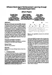
We can see how DOORMAX not only learns with significantly less sample complexity, but also how well it scales to the larger problem. After increasing the number of states by more than 14 times, DOORMAX only requires 1.55 times the experience. The main difference between DOORMAX and FactoredRmax is their internal representation, and the kind of generalization it enables. After just a few examples in which ¬touchN (taxi, wall) is true, DOORMAX learns that the action North has the effect of incrementing taxi.y by 1, whereas under touchN (taxi, wall) it fails. This knowledge, as well as its equivalent for touchS/E/W , is generalized to all 25 (or 100) different locations. Factored-Rmax only knows that variable taxi.y in state s depends on its value in state s, but still needs to learn the transition dynamics for each possible value of taxi.y (5 or 10 different values). In the case of actions East and West, it’s even worse, as walls make taxi.x depend on both taxi.x and taxi.y, which are 25 (or 100) different values. As DOORMAX is based on interactions between objects, it learns that the relation between taxi and wall is independent of the wall location. Each new wall is therefore the same as any known wall, rather than a new exception in the movement rules, the kind Factored-Rmax needs to learn. 6.2. Pitfall Pitfall is a video game released in 1982 by Activision for the Atari game console. The goal is to have the main character (Man) traverse a series of screens while collecting as many points as possible while avoiding obstacles (such as holes, pits, logs, crocodiles and walls) and under the time constraint of 20 minutes. All transitions in Pitfall are deterministic. Our goal in this experiment was to have the Man cross the first screen from the left to the right with as few actions as possible. Figure 2 ilustrates this first screen. Our experiments were run using a modified Atari emulator that ran the actual game and detected objects from the displayed image. We used a simple heuristic that identified objects by color clusters and sent joystick commands to the emulator to influence the play. For each frame of the game, a list of object locations was sent to an external learning module that analyzed the state of the game and returned an action to be executed before the emulator continued on to the next frame. If we consider that we start from screen pixels, the flat state representation for Pitfall is enormous: 16640x420 . By breaking it down into basic objects, through an object recognition mechanism, the state space is in the order of the number of objects to the number of possible locations of each object: 6640x420 . OO-MDPs allow for a very succint representation of the problem, that can be learned with only a few experience samples.


7. Conclusions and Future Work

Figure 2. Initial screen of Pitfall.

The first screen contains six object types: Man, Hole, Ladder, Log, Wall and Tree. Objects have the attributes x, y, width and height, which define their location on the screen and dimension. The Man also has a Boolean attribute of direction that specifies which way he is facing. We extended the touchX relation from Taxi to describe diagonal relations between objects, including: touchN E (oi , oj ), touchN W (oi , oj ), touchSW (oi , oj ) and touchSE (oi , oj ). These relations were needed to properly capture the effects of moving on and off of ladders. In our implementation of DOORMAX, we defined seven actions: WalkRight, WalkLeft, JumpLeft, JumpRight, Up, Down and JumpUp. For each of these actions, however, the emulator has to actually execute a set sequence of smaller frame-specific actions. For example, WalkLeft requires four frames: one to tell Pitfall to move the Man to the left, and three frames where no action is taken to allow for the animation of the Man to complete. Effects are represented as arithmetic increments or decrements to the attributes x, y, width, height, plus a constant assignment of either R or L to the attribute direction. The starting state of Pitfall is fixed, and given that all transitions are deterministic, only one run of DOORMAX was necessary to learn the dynamics of the environment. DOORMAX learns an optimal policy after 494 actions, or 4810 game frames, exploring the area beneath the ground as well as the objects en route to the goal. Once the transition dynamics are learned, restarting the game results in the Man exiting the first screen through the right, after jumping the hole and the log, in 94 actions (905 real game frames), which is what the optimal policy requires. A few examples of the (condition, effect) pairs learned by DOORMAX are shown below: Action WalkRight

Condition direction = L

WalkRight JumpRight Up

touchE (Man, Wall) direction = R on(Man, Ladder)

Effects {direction = R, Δx = +8} no-effect Δx = +214 Δy = +8

We introduced OO-MDPs, an object-oriented representation for reinforcement-learning problems that provides a natural way of modeling a broad set of domains, while enabling generalization. We presented DOORMAX, a learning algorithm for deterministic OO-MDPs that not only outperforms state-of-the-art algorithms for factored-state representations, but also scales very nicely with respect to the size of the state space, as long as transition dynamics between objects do not change. We presented bounds for learning transition dynamics of determinstic OO-MDPs in the KWIK framework. One limitation of our work is that we do not yet have a provably efficient algorithm for stochastic domains, which is part of our future work. While OO-MDPs can model stochastic transitions, a more complex learning algorithm would be needed to learn transitions effectively in the face of noise. The second component of our future research is the extension of the object-oriented model to be able to handle inheritance. We hope to be able to exploit knowledge about objects being part of a common super-class to learn their behaviors faster. Ideally, algorithms could also learn the object definitions and classes automatically, as well.

References Boutilier, C., Dean, T., & Hanks, S. (1999). Decision-theoretic planning: Structural assumptions and computational leverage. Journal of Artificial Intelligence Research, 11, 1–94. Dietterich, T. G. (2000). Hierarchical reinforcement learning with the MAXQ value function decomposition. Journal of Artificial Intelligence Research, 13, 227–303. Guestrin, C., Koller, D., Gearhart, C., & Kanodia, N. (2003). Generalizing plans to new environments in relational mdps. IJCAI (pp. 1003–1010). Li, L., Littman, M. L., & Walsh, T. J. (2008). Knows what it knows: A framework for self-aware learning. Twenty-Fifth International Conference on Machine Learning. Puterman, M. L. (1994). Markov decision processes—discrete stochastic dynamic programming. New York, NY: John Wiley & Sons, Inc. Strehl, A. L., Diuk, C., & Littman, M. L. (2007). Efficient structure learning in factored-state mdps. AAAI (pp. 645–650). AAAI Press. Sutton, R. S., & Barto, A. G. (1998). Reinforcement learning: An introduction. The MIT Press. van Otterlo, M. (2005). A survey of reinforcement learning in relational domains (Technical Report TR-CTIT-05-31). CTIT Technical Report Series, ISSN 1381-3625.