DATE OF REPORT (Yeer, #onth, Day). 15. PAGE COUNT. Technical. FROM ..... begins another pass at moving the simulated vehicle toward its go-al. 14 ...... A map database of the ALV test site has been constructed by the U.S. Army. _.
AD-RIBS 166
UNCLASSIFIED
AN OVERVIEW OF VISION-BASED NAVIGATION FOR AUTONOMOUS VEHICLES 1966.. (U) MARYLAND UNIV COLLEGE PARK CENTER FOR AUTOMATION RESEARCH S CHRNDRAN ET AL. AR 67 CAR-TR-265 ETL-6479 DAC76-84-C-6664 F/G 12/9
1/'2 NL
EIhEEEEllljI //I/IElUll/I/E EEEIIIIIIIIEEEE llmllllllEllE llEEllllllllEE /hI///EE//lEEI
r.
1111.0
~
IIIII
~"-
L
2=
28
112.2
1.4
MICROCOPY RESOLUTION TEST CHART NATIONAL BUREAUOF STANDARDS-I963 A
1 -
'w
'
.
.
-
-
, .,
-
-W .
.
W
, --. ,"
w
ETL-0479
UiC FILE COD,
An Overview of Vision-Based Navigation for Autonomous Land Vehicles 1986 AD-A188 186 Sharat Chandran Larry S. Davis Daniel Dementhon Sven J. Dickenson Suresh Gajulapalli Shie-Rei Huang
Todd R. Kushner Jacqueline LeMoigne Sunil Puri Tharakesh Siddalingaiah Phillip Veatch
Center for Automation Research University of Maryland College Park, Maryland 20742
April 1987
DTIC DEC 0 7198
APPROVED FOR PUBLIC RELEASE; DISTRIBUTION IS UNLIMITED.
Prepared for
U.S. ARMY CORPS OF ENGINEERS ENGINEER TOPOGRAPHIC LABORATORIES FORT BELVOIR, VIRGINIA 22060-5546
017
'9
ZTI
s
Destroy this report when no longer needed. Do not return it to the originator.
The findings in this report are not to be construed as an official Department of the Army position unless so designated by other authorized documents.
The citation in this report of trade names of commercially available products does not constitute official endorsement or approval of the use of such products.
WTI %i
'S.
"S4.fw.,
~
.
~, .p4*",
S.".
S
.
I
UNCLASSIFIED ECURITY CLASSIFICATION OF THIS PAGE Form Approved
REPORT DOCUMENTATION PAGE la. REPORT SECURITY CLASSIFICATION
.
OMB No 0704.0188
lb RESTRICTIVE MARKINGS
UNCLASSIFIED
N/A
Za. SECURITY CLASSIFICATION AUTHORITY i4b. C/
3. DISTRIBUTION IAVAILABILITY OF REPORT
Approved for public release;
DECLASSIFICATIONDOWNGRADING SCHEDULE N/A
distribution unlimited
. PERFORMING ORGANIZATION REPORT NUMBER(S)
S. MONITORING ORGANIZATION REPORT NUMBER(S)
CAR-TR-285 ETL-0479
CS-TR-1831 6a. NAME OF PERFORMING ORGANIZATION f
6b. OFFICE SYMBOL
l(If
applicable)
University of Maryland
7a. NAME OF MONITORING ORGANIZATION U.S. Army Engineer Topographic
N/A
%
Laboratories
6c. ADDRESS (City, State, and ZIP Code)
.
7b ADDRESS (City, State, and ZIP Code)
Center for Automation Research Fort Belvoir, VA 22060-5546
College Park, MD 20742-3411 Ba. NAME OF FUNDING/SPONSORING
Defense
ORGANIZATION
Advanced
8b OFFICE SYMBOL (if applicable)
-Research Projects Agency
ISTO
9 PROCUREMENT INSTRUMENT IDENTIFICATION NUMBER
DACA76-84-C-0004 10 SOURCE OF FUNDING NUMBERS PROGRAM IPROJECT TASK NO. NO. ELEMENT NO.
ADDRESS (City, State, and ZIP Code)
1400 Wilson Boulevard
623013E
Arlington, VA 22209
WORK UNIT
I
I
ACCESSION NO.
11. TITLE (Include Security Clasification)
An Overview of Vision-Based Navigation for Autonomous Land Vehicles 1986
2.PERSONAL AUTHOR(S) S. Chandran, L.S. Davis, D. Dementhon, S.J. Dickenson, S. Gajulapalli, .R. Huang, T.R. Kushner, J. LeMoigne, S. Puri T. Siddalingaiah, and P. Veatch 3a. TYPE OF REPORT
13b. TIME COVERED FROM
Technical
14. DATE OF REPORT (Yeer, #onth, Day)
15. PAGE COUNT
117
April 1987
TO NIA
16. SUPPLEMENTARY NOTATION
17.
COSATI CODES
FIELD
GROUP
17 09
07 02
SUB-GROUP
18. SUBJECT TERMS (Continue on reverse ifne rsseary and identify by block number)
Vision-Based Navigation,,. Parallel Algorithms, .
'19. ABSTRACT (Continue on reverse ifnecessary and identify by block number)
K.
This report describes research performed during the first two years on the project Vision-Based Navigation for Autonomous Vehicles being conducted under DARPA support. The report contains discussion of four main topics:
1) Development of a vision system for autonomous navigation of roads and road networks. f2) Support of Martin Marietta Aerospace, Denver, the integrating contractor on DARPA's ALV program. "3) Experimentation with the vision system developed at Maryland on the Martin Marietta ALV. Development and implementation of parallel algorithms for visual
4)
navigation on the parallel computers developed under the DARPA Strategic Computing Program--specifically, the WARP systolic array processor, the Butterfly, and the Connection Machine. . . 0.DISTRIBUTION IAVAILABILITY OF ABSTRACT I3 UNCLASSIFIED/UNLIMITED 93 SAME AS RPT .2a. NAME OF RESPONSIBLE INDIVIDUAL
0
DTIC USERS
21. ABSTRACT SECURITY CLASSIFICATION UNCLASSIFIED ,, 22b TELEPHONE (Include Area Code) 22c. OFFICE SYMBOL
an (o hk355-2767
SDForm 1473,
JUN 86
Previous editions are obsolete.
.,"
ETL-RI-T SECURITY CLASSIFICATION OF THIS PAGE
UNCLASSIFIED -
'***
-
P
?*$*%
TABLE OF CONTENTS PAGE iv
List of Figures and Tables 1. Introduction
1
2. Simulation Systems
6 6 8 12
2.1 Vehicle simulator 2.2 Structured light ranging system 2.3 Range simulator
16
3. Visual Navigation System
16 16 20 20 20 23 25 33 37 39 43 44
3.1 Introduction 3.2 Vision executive 3.3 Image processing 3.3.1 Video image processing 3.3.1.1 Thresholding algorithms 3.3.1.2 Multiresolution algorithms 3.3.2 Range data processing 3.4 Geometry module 3.5 Map database 3.6 Predictor 3.7 Sensor control 3.8 Representation
46
4. Path Planning
47 52
4.1 Multiresolution representation based path planning 4.2 Experimental results 5. Rule-Based Visual Navigation
53
6. Butterfly Algorithms
58 58 60 61 64 66 67
6.1 The Butterfly parallel processor 6.2 Butterfly Hough transform 6.2.1 Computing the Hough array 6.2.Z Implementation details 6.2.3 Peak detection 6.3 Parallel search 7. Experimental Results
8.
r.. %
70
7.1 Simulator experiments 7.2 Experiments at Martin Marietta
70 71
References
74 iii
:-44
.,.
FIGURES AND TABLES TITLE
FIGURE
PAGE
1.1
System configuration
2a
2.1
ALV simulator
8a
2.2
Plane-of-light range scanner mounted on robot arm
8b
2.3
Creation of a range table from images of light stripes
9a
2.4a
Range image in camera system
9b
2.4b
Range image in mirror system
9b
2.5
Simulated visual imagery
15a
2.6
Typical range image (derived from time 3)
15b
2.7
Key for obstacle maps
15c
2.8
Obstacle map at time 0
15d
2.9
Obstacle map at time 1
15e
2.10
Obstacle map at time 2
15f
2.11
Obstacle map at time 3
15g
3.1
Thresholding algorithm applied to an image from the Martin Marietta test site
21a
-
3.2a
The second thresholding algorithm applied to an image from the Martin Marietta test site
a 22a
-
3.2b
Same algorithm as 3.2a applied to an image with contrast reversal A third algorithm applied to an image with contrast reversal
22a
3.2c
22b
3.3
Multiresolution algorithm applied to an image from the Martin Marietta test site
3.4 3.5a
Range scanner geometry Range images of an obstacle on a road
32b
3.5b
Video image of obstacles on roads
32c
b
3.6a
Thresholded 0 derivatives
32d
..
3.6b
Thresholded 0 derivatives of first montage Method for the reconstruction of the road from an image
32d 33a
'-.
3.8
Sequence of 4 images, reconstruction by flat earth assumption, and 2 views of 3-D reconstructions by zero bank algorithm
35a
3.9
Basic principle of prediction with flat earth assumption
39a
3.10 4.1
Image from C l, top view of the world, image from C2 (Method A), and 42a image from C2 (Method B) A path is planned: Path planning time, cost function, and path analysis time 52a
4.2
A new path is planned: Path planning time and cost function
3.7
iv
24a 25a
,: $
..,.
52b
7'.
53a
5.1 5.2
Scene model builder dataflow Road patch and planar ribbon frames
54a
5.3 5.4
Top-down hypothesis generation Bottom-up hypothesis generation
55a 56a
7.1 7.2
Curving road Detected boundaries
69a 69a
7.3 7.4
Road image from next vantage point with sensor control Same as Figure 7.3, but without sensor control
70a
7.5
Intersection
71a
7.6a
Forbidden region and prediction windows
71b
7.6b
Extracted road boundaries
71b
7.7
Image from next vantage point
71c
70a
TITLE
PAGE
3.1
Comparison of obstacle detection algorithms for sensitivity to scanner
32a
6.1
Parallel search processing times
68a
TABLE
I,,
"
GN
PAGE
TITLE
FIGURE
7. ?,
-F or
.1i,
vv
L." - t-
I ft S
Sf
. . . -'- 5.. -
t
,.*
1. Introduction
This report describes research performed during the first two years on the project Vision-Based Navigation for Autonomous Vehicles being conducted under DARPA support. Our project, to date, has focused on four goals:
1)
Development of a vision system for autonomous navigation of roads and road networks.
2)
Support of Martin Marietta Aerospace, Denver, the integrating contractor on DARPA's ALV program.
3)
Experimenting with the vision system developed at Maryland on the Martin Marietta ALV.
4)
Development and implementation of parallel algorithms for visual navigation on the parallel computers developed under the DARPA Strategic Computing Program-specifically, the WARP systolic array processor, the Butterfly and the Connection Machine. We have constructed, in our laboratory, a simulation facility for developing
our visual navigation system. This facility consists of a robot arm carrying a sensor package over a terrain board. Roads and road networks are painted on the terrain board. The sensor package includes a black and white solid state camera, a structured light range scanner that provides range data registered with the black and white video data, and position encoders that allow us to control the height and attitude of the image sensors with respect to the terrain board. The simulation facility is described in greater detail in Section 2.1. While the imagery produced by the sensors on the robot arm is quantitatively different from data collected by the sensors on the ALV at Martin Marietta, we have found this simulator to be very valuable in designing the control components of the navigation system; these components account for the larger part of the actual code in
..
S'
Ss_
s
the system. We have also developed a software simulation system for range data
--
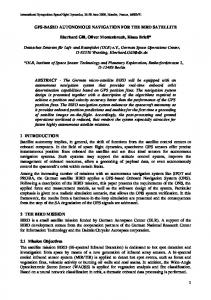
analysis. The simulator generates range images of a three dimensional polyhedral world. It is described in Section 2.2. Section 3 of this report provides an overview of our visual navigation systern. Figure 1.1 is a block diagram of the principal components of that system. The organization of the system was originally described in Waxman et al. Ill.
-
The vision executive controls the activities of the other modules in the system. Its principal responsibilities are:
1)
Controlling the focus of attention mechanism for image processing (i.e., identifying subsets of the sensed data likely to contain critical features for navigation and predicting both the photometric and geometric properties of these features).
2)
Using knowledge stored in its visual knowledge base both to verify the model of its environment constructed on the basis of analyzing previous images and to extend that model further in the direction of travel.
The vision executive is described in more detail in Section 3.2. The image processing module (Section 3.3) contains algorithms for extracting structures from the image data that potentially correspond to objects of interest in the scene,
,.
such as boundaries of roads or obstacles on roads. The geometry module (Section 3.4) contains a variety of methods for reconstructing the three-dimensional geometry of the scene. The vision executive chooses the appropriate reconstruction technique either based on a priori knowlcdge about the environment or from
2 tit
IMAGE PROCESSING Bootstrap and Feed-Forward Modes
DISUAL KNOWLEDGE BASE Rules & Models
- Linear Features - Gray segmentation - Color analysis J
3-D
GEOMETRY 3-D SHAPE RECOVERY -
Road structures - Obstacle models - (Object model) -
\
2-D symbols &4 interpretation
2-D symbols
-
Monocular inverse perspective Active ranging (Stereo)
scene model 2-D
*
4--mode & windows
groupings-
4-3-D
interpretation
' scene modell 3-0 SCENE REPRESENTATION 3-D
DISION EHECUTIVE OVERALL VISION PROCESS O NTROL sceneprediction & windows
-
SC ENE PREDICTOR 3-D
pointing
SENSOR CONTROL
verification
and
extension
,
-
representation
~posit
&ll~
map daarequests3-\rp
o
NAVIGATOR
requests
BASE
- Spatial
A
Terrain data base ds Jcomman surveillance [ (Landmarks)
-
ii n,
IOL
__' DATA
representation
poitin
Focus of attention mechanismns
-Model
position & L
j
[Istatus
trajectory
- Temporal
__/
trajectory
goals p ri o ri t i e s s t a t u s priorities -s t'atus
S re q u e s t s &
~
~~pdating
terrain data
"
travel
path
PLANNER
location goals
Goal specification -
Priorities
-
Resource
PILOT allocation
-
Path interpreter Dead rcckoning Inertial navigation
Figure 1.1 System configuration
..........
:-:
its analysis of previously sensed data. During the past several months we have extended the navigation system so that it can navigate over networks of roads. We have done this by incorporating
e
a map database (Section 3.5) that includes a map of the roads on the terrain board. The organization of this database is identical to that of the road network map compiled by ETL for the Martin Marietta test site. The map is used by an extended scene prediction module (Section 3.6) to provide the vision executive with predictions about the appearance of the road(s) in its field of view. These
%
predictions not only allow the vision executive to control its focus of attention mechanism, but also to control the viewing directions of its sensors to ensure that critical scene features are in their field of view (Section 3.7). The planning module not only develops a prior route plan from the road map but also plans the local path of the vehicle through the three dimensional model constructed by the vision executive. Until now, this has been straightforward since our roads did not contain any obstacles.
In more complex environ-
ments, of course, the planning problems become much more severe.
We have
developed a path planning system that utilizes a multiresolution representation of free space, obstacles and unknown space (shadows of obstacles and parts of the environment beyond the field of view of the sensors) that should be applicable to
%
relatively complex planning problems. This path planning system is describe(d in Section 4. Our experience with the system described in Section 3 has made it clear that a more flexible framework is needed, principally for specifying the control aspects 3! 3:Z..."
of navigation. For example, our current system has a single strategy for tracking the boundaries of the road in an image-the scene prediction module identifies windows near the bottom of the image that will contain the projections of the left and right road boundaries, and after the image processing module identifies the actual locations of the projected road boundaries in those windows. Subsequent windows are placed that allow us to continuously track the road boundaries through the image. However, it would sometimes be advantageous to use some other strategy for tracking the road. For example, if prior knowledge indicated that the stretch of road currently being traversed were straight then one could imagine a strategy where after the initial windows were processed subsequent windows were placed relatively high up in the image, corresponding to segments of road relatively far from the vehicle. These and similar considerations have led us to design and develop an object-oriented system for visual navigation.
A ..
description of this system is included in Section 5. One of the principal goals of the DARPA Strategic Computing Program is to understand how different models of parallel computation can be applied to problems in artificial intelligence.
Towards this end, DARPA has sponsored both the
hardware and software development of a variety of parallel machines, including the WARP[2], the Butterfly[3] and the Connection Machine[4].
The Computer
Vision Laboratory currently has both a 16 processor Butterfly and a 128 processor Butterfly. A WARP is scheduled for delivery sometime during 1987. In
November of 1985,
Todd Kushner spent several
weeks at Martin
Marietta, Denver, installing a version of our visual navigation system on the AIA'
.
(these and other experiments are discussed in Section 7). Based on these experimeits, we made certain modifications to the design of that system and then froze the design during the winter of 1986.
Since then we 'have been working on a
Butterfly implementation of most of the major components of that system. The Butterfly system performs the following operations in parallel: I
window placement
2)
Hough transforms for linear feature extraction (here we assume that the lowest level of visual processing is done on a machine such as the WARP and consider only the clustering aspects of linear feature extraction)
3)
monocular inverse perspective search for an acceptable scene model
4)
Section 6 contains a description of the Hough transform Butterfly implementation, as well as some recent work on parallel search algorithms. Finally, we have conducted a series of experiments both in the laboratory
'-. ,
and on the Martin Marietta ALV. In Section 7.1 we describe recent experiments that involve navigating the robot arm through and into intersections, and in Section 7.2 we describe experiments performed on the ALV both in November 1985 and August 1986.
.. %
.%
2. Simulation Systems In this section we describe the laboratory facility that we have constructed to support the development of algorithms for visual navigation. Section 2.1 contains a description of the vehicle simulator, Section 2.2 describes the structured light range sensor, and Section 2.3 describes a range data simulation program.
2.1 Vehicle simulator
The vehicle simulator is a system which reproduces at reduced scale the interactions between the motion and the resulting changes in visual environment of a full-scale vehicle.
The four components of the system are:
1.
A terrain model board, modeling the landscape that the robotic vehicle is likely to encounter;
2.
A camera, positioned with respect to the terrain model in the same fashion as the vehicle camera would be positioned with respect to the world terrain;
3.
A structured light ranger, designed to model the laser ranger of the vehicle and give images containing depth information;
4.
A robot arm, which displaces the sensors across the terrain board in response to sensor data analysis software in the same fashion as the propulsion system of the full-scale vehicle would displace the vehicle sensors.
.,:
More details are now given about these four components of the simulator.
The robot arm is an American Robot arm, with six independent axes of movement, waist, shoulder, elbow, wrist (two axes), and tool. The motion of the tool plate has an accuracy of 1/1000 inch.
I".
The arm is controlled by seven microprocessors; a Motorola 68000 processor supervises the six Motorola 6809 motion control processors. They interface with the user through the Magix operating system, a UNIX look-alike.
The arm can
be programmed with a specific robotic language, AR-BASIC, which also includes commands for communications with other computers such as the VAX computers of our laboratory. The terrain model is constructed on a 4' X 41 board.
It models several
paved road surfaces on various straight lines, s-curves, hills and intersection
I,
configurations. The camera-ranger system is displaced along these road segments by the robot arm, whose motions are computed by the programs run on the VAX computer on the basis of the image and range data that are gathered by the camera and the ranger and processed by the VICOM image processor. The camera mounted on the robot arm is a Sony CCD array black-andwhite camera. The camera images are input to a VICOM image processor controlled by a Motorola 68010 processor, or to a GRINNELL image processor controlled by a VAX 11/785 computer. Mounted on the sides of the camera are three linear compression encoders which are used to maintain height, pitch, and roll of the camera in relation to the corresponding quantities of the simulated robotic vehicle.
The signals from
these encoders are processed by three of the seven analog-to-digital converters available with the robot arm hardware.
.%
%
2.2 Structured light ranging system
The technology of laser rangers small enough to be mounted at the end of a robot arm is not available yet. Meanwhile a plane-of-light range scanner has been built to provide similar information and functionality.
0,
Its frame is mounted on
the end plate of the robot arm, and supports the camera (Figure 2.1). Figure 2.2 shows more details of the structure of the plane-of-light range scanner and its mounting with respect to the camera and the robot arm. The 150 W light generator is mounted on the robot arm itself and is not shown. The light is brought to the scanner by a four foot fiber optic light guide, which flares to a fine line of fibers. The line of light from the fiber optics line is further narrowed by a 4/1000 inch slit. The diverging light from this slit is refocused to a plane of light by a cylindrical lens. The plane of light is redirected out of the box of the device by a three-inch long mirror, whose angle is precisely controlled by a geared-down stepper motor.
The stepping motor is connected to the VICOM
computer through a controller card, and the command "STEP" from a VICOM displacement Pascal program rotates the motor one step, giving a mirror angular
N
of 0.045 degrees. A full mirror revolution takes 8000 step commands. The plane of light intersects an object in a planar world curve, and the image of this curve is seen from the camera. This image curve has a thickness of several pixels, and the median line of this curve is obtained. Each row of the image for a given position of the mirror is the image of a straight world line with a specific distance to the axis of the mirror, as shown in Figure 2.2.
A two.5.ia
Robot
arm
Terrain
board
-~ %
Figure 2.1 ALV simulator
Ohl
Robot armi mounting plate
Lens
Ligh gude I
ceterRange
matrix 0i,j)
Camera
Figure 2.2 Plane-of-light range scanner mounted on robot arm
-VA 4%A-W.%
dimensional lookup table is calculated to give the ranges of all the world lines
k
within the camera field of view and the mirror field of range. This lookup table maps the ranges of the intersection lines shown as dots in Figure 2.2. The range acquisition algorithm is illustrated in Figure 2.3 and proceeds as follows: 1.
While the mirror is at its home position facing the lens, a camera frame is grabbed. This is the initial image.
2.
The mirror is moved from its home position to the initial scanning angle.
3.
A camera frame is grabbed, which may contain the image of the intersection of the plane of light with a world object.
4.
The difference between this image and the initial image is taken. Most of
the information out of the image of the illuminated stripe is removed by this differencing operation. 5.
The maximum brightness of the image of the stripe is calculated.
6.
The image is thresholded to set the gray levels to zero out of the stripe (top right image of Figure 2.3).
7.
Each image column is scanned until a non-zero pixel corresponding to a stripe boundary is found, then scanned further until a zero pixel corresponding to the other boundary is found. The row of the midpoint is calculated. The range of this pixel is found in the range lookup table at the appropriate mirror step column and pixel row line. The resulting range is placed in the range image being built, at the row indexed by the mirror steps, and column indexed by the image pixel column.
8.
When all the image columns of a stripe image obtained for a given mirror step have been scanned, the row of the range image corresponding to this given mirror step is full, and the mirror is displaced to the next step. The program loops between items 3 to 8 until the stripe for the maximum step angle has been processed.
9.
.0 1
%-%
When the range image acquisition is completed, it is displayed, and the mirror completes its rotation up to its home position facing the lens. • ,%,,..
Thresholded
pixel row
im
e
j-
image
range
strie
column
k
to mro a__
Range
_4-
IookuR table
mirror
step
i --0*----4
Raigie
a~
Figure 2.3 Creation of a range table from images of light stripes
]W
a
I
'I.
p ~m.
.'... 4.4... .'.-
~. 5,.,
va~.
V.
a
Figure 2.4a Range image in camera system *~5~5*
*5* 5.,. S-p.....
I.p-p S.' ~*555
*~ **5 4..
-V. ~ via
4
Figure 2.-lb Range image in mirror system
4..
SW
-
~
*U~
.A
j~S
LUX
Notice that this method for constructing the range is different from other structured light approaches.
Previous work on structured light rangers con-
structed the range image in the camera coordinate system. Such a range image is shown in Figure 2.4.a. This image contains a spool of thread on a ground plane, with a vertical plane in the background. In such a range image, pixels between the images of the stripes are black because no range information could be obtained. It would be difficult to eliminate these gaps between the stripes without also smoothing the significant range discontinuities corresponding to the presence of object edges. In the method proposed here, the problem of the gaps between stripes has
%mJ
been eliminated. The image construction method is based on the observation that if we position a camera with its lens center on the mirror axis, such a camera would see all the stripes as straight lines, even for stripes that the other camera sees as ellipse segments, because the images of the stripes with this new camera are contained in the plane of light which produces them. Straight stripe images obtained for different mirror steps are parallel and can be compressed to eliminate the gaps and build a continuous range image. Actually, a second cam*1%
era is not required, since enough information from the original camera and mirror position is available to synthesize a range image as seen from the mirror's point of view. After stripe thinning, each straight stripe would be one pixel thick, so that each pixel row of the final image would correspond to a different stripe and therefore to a different mirror step. The range from a world point to the mirror can be obtained for each straight stripe pixel by the same triangulation procedure 10
which produced the range to the original camera. The range image acquisition algorithm presented above implements the proposed method and produces a range image from the mirror point of view. Figure 2.4b is a range image obtained by this method for the same scene as Figure 2.4a. The spool looks more compressed because the aspect ratio of the picture depends on the mirror step angle, and also because the mirror was higher above the spool than the camera. Consequently the upper face of the spool and its holes are more visible. A laser ranger would give a similar picture, because one picture row would also be obtained for each step of its vertical-scanning mirror.
However, there
would not be any shadow behind the spool. A shadow occurs in the structured light image because a part of the stripe of light was hidden from the camera by the spool, which prevented range calculation.
..
.p-
NO
N% 11
2.3 Range simulator As an alternative to driving an ALV or directing a robot arm about a terrain board, we have developed an image synthesizer that allows us to create a world of objects and obtain range and visual images from any viewpoint in this world. The ability to make images from arbitrary positions is exactly equivalent to gathering images from an ALV that is driving through the synthetic world. The synthesizer can model spheres, parallelepipeds, planar surfaces, cones, and cylinders. These objects can be translated and rotated in any fashion and may be positioned so that an object is partially or wholly inside of another object (an important property when constructing complex scenes from these basic building blocks). After each object has been positioned (by multiplying it by a transformation
-,,
matrix), a visual image is calculated based on a perspective projection in which the focal point is at the origin of the coordinate system and the image plane is placed in front of it at z = focal length. Each pixel in the visual image has associated with it a grey level and a zdistance.
The grey level can be created with the light source at any position.
Surface reflections are assumed to be Lambertian and all objert.s have an equal albedo (it would be a simple ext ension to add variable all
,Is,). No comr pensa-
tion is made for lowering intensity due to increawsed di-tancc from the iinage
plane and the light source. ... '
12
% %
%
IL From the visual image and the corresponding z distances we can calculate what the range image would appear to be.
This initial range image has pixels
that are spaced at equal intervals on the image plane. However, the BRIM range
-
scanner produces images that are at equal angular intervals on the image plane so we convert to this format in order to accurately simulate the ALV's range scanning process. Interpolation of the initial range image is done using an intentionally crude algorithm to introduce noise into the system (of course, simply digitizing the image of the objects has introduced some noise, particularly for objects that have high curvature such as spheres). The final equiangular range image has all of the properties of an image produced by an ERIM scanner mounted on an AIV including the same field of view, eight-bit range values, and 61-foot anibi%
guity intervals. The obstacle detection algorithms described in Section 3.3.2 are applied to
,'
the equiangular range image and the resultant binary obstacle image is mapped from spherical coordinates into the cartesian x-z ground plane.
The ground
plane map has initially four types of pixels: 1) obstacles or unnavigable terrain, 2) traversable terrain, 3) areas whose traversability is unknown because they are hidden by an obstacle (i.e.: shadow regions), and I) areas whose traversability is unknown because they are outside of the field of view of the siiliilnted laser sen-
",'
'I
sor. The path planner will treat the ALV as if it were the size of :i single pixel so
-
a boundary the width of the ALV's radius is grown around all o,tacle and shadow pixels.
13
W
%
At the start of the simulation the program requests the coordinates of the ultimate goal for the ALV. A straight line from the current location to this goal is plotted and a move along it is calculated.
The endpoint of the move is passed
to the path planner which tries to find a path through the ground map from the current location to the endpoint.
The path planner uses a hierarchical algorithm
based on a quadtree division of the ground map. The planner assumes that the vehicle can only travel through pixels that are marked a.s traversable. a..
If the planner fails to find a path to the first endpoint a series of heuristics are used in sequence to select alternate subgoal locations. Each subgoal is passed, one at a time, to the path planner until one is found that can be reached.
If all
of the heuristics are exhausted without a reachable subgoal being found, the program notifies the user and gracefully terminates. Once the endpoint of the next move is found a transformation matrix is calculated that will place the origin of the coordinate system at this new location. This matrix, when applied to each object, will result in the next visual and range images being the scene that an ALV would see if it were driven to the endpoint. The matrix is fashioned so that the vehicle will be facing the ultimate goal location (other constraints on what direction the vehicle should be facing or how long each move should be are adjustable parameters in the program).
If the move's
endpoint is the same as the goal location the program terminates. Otherwise the transformation matrix is applied, the new visual image is found and the program begins another pass at moving the simulated vehicle toward its go-al.
14
Figures 2.5 - 2.11 show some output from a typical simulation in which the modeled ALV drives approximately 200 feet to reach a goal location. There is no limitation on the distance from the starting point to the goal in the simulation.
I,'.,
Figure 2.5 shows the visual images synthesized while traveling past several obstacles. A typical range image is shown in Figure 2.6. Figure 2.7 provides a key for Figures 2.8
-
2.11.
These latter figures are the ground maps produced from the
final range images at each step. Each map covers approximately 65000 square feet. The vehicle's current position is always at the center of the map.
.
%4,
%
)1 -4
TIME*~
ze
TIE
04
FO4
2TIME
TIME
Figur
2.5
Siuae
viua
imaer
f%
.. . -S
) image derived from time Figure 2.6 Typical range
.'.
.
*1
1! *
OUTSIDE OF THE SCANNER'S FIELD OF VIEW '4'
NAVIGABLE REGION
n.
GROWN BOUNDARY REGION
OBSTACLE REGION
SHADOW REGION
Figure 2.7
Key for obstacle maps
'
."2
..
.
..,,:
.4.
p.. S.
a-N'
m's N
$ h
/
A~/
//4;$
~/4 4.
a.4.
a%.a-
N.. St.
p
S. ~a
Sj,*
S.
A
.4..
.~SJS
-a-.
ND
~55*
S.
Figure 2.8 Obstacle map at time 0
S%~~j
a.
lSIS.J*~
I Sr
ND.
.P
~
-
--
.
--
.-
-....
I
~. a, a,
a, a,
a
a, a'
'~'.
--
a, ad
'a.'
*
'-a,
Figure 2.9 Obstacle map at tune 1
a
J.
H p
p.
Np
"p. "p. "Np
"p4
A. *
a~*
"'S *45
"p. -'S
4-
-S 5~4~
*
"p4
'"S
h
U
Figure 2.10 Obstacle map at time 2 'S
'S
I
'-p.. a,.
'.5.
* p. 'S
S.
p
4.
.9 2\~~
S
.~
I
S
S
S
figure '2.11
Obstacle tnaT at time i
S
S
3. Visual Navigation System
3.1 Introduction This section contains an overview of the visual navigation system. This systern runs on a VAX/VICOM environment, with image acquisition and some low level processing being done on the VICOM and the remainder of the vision processing, planning and navigation being performed on the VAX.
4"
3.2 Vision executive The principle responsibilities of the vision executive are:
1) controlling the focus of attention mechanism for sensor data processing, and 2) verifying and extending the sensor-based model of the environment. Both of these tasks involve sensor control (for example, determining the appropriate pan and tilt for the video cameras), map database analysis and geometric reasoning about the three dimensional properties of scene objects identified in the sensor data. Consider, for example, the verification of that portion of the scene model not yet traveled-i.e., still in front of the vehicle.
''',
Due to limitations of the vision
and navigation systems this model will, to some degree, be inaccurate.
Both to
reduce these inaccuracies and to provide an anchor for analyzing previously unexplored parts of the scene, the vision executive analyzes those parts of the sensed data expected to contain components of the scene model.
In order to do this, the
vision executive must first decide, before acquiring an image, what parts of the
%
% Y18' 4.
'' 4"
S
V
--
.
-~~%
4%
scene model it will search for. Then. ba.sed on the three dinieinsii:l prprtie, ('
the scene model and a model for tie assulned model,
nIotioln of
the vliejh, throh 11
-t-
it can determine a viewing angle for the eaniera thatt will I,',luee' :ll
image that will include those corn ,,nents. (urrently
thi-s is ,(iw h Itryiigr
center the field of view of the camera oin a point in the center
t,,
f the i):il :tfixed
distance in front of the vehicle. The (listale cho ,el i.a filiiitilr o4, 1,lt 1 v,'leich" d (h)uie speed and the extent of the ciurrent three dimenrsohnadil ro,o, ri,,hIl.
ciIdl
imagine, of course, more sophisticated strategies for camera coitrol 1, (",oil other visual goals. The details of the sensor control module are colit aiiicd ill Seetion 3.7. Once the direction of view of the camera is established, the vision ex('i'tive can work with the scene predictor to establish the projected positions of key In the current imlplementation. the fIl-
scene features in the next image frame. lowing types of predictions are supported:
1) Identify the points on the boundary of the image where th lel't :11,t riilt road edges will enter the image. 2)
Given a point x feet in front of the vehicle on the left (ri~lit ) l ,1lil:,rv the road, will that point appear in the imnge and, if so,. ,,,r,.
-
()f
The vision executive then places rectangular windows arouit these prelicti on., and sends those windows to the appropriate sensor dat a p r cv.*ii extract the corresponding image object (straight edge segients
,
li,,
f p'iti' uri,.i :-
-r'
tion and contrast sign for ;dentifying rod bomi:,rivs).
17
-
% ..
%.
Currently', the "verification" stage of processing ends after thie firstI h%() willdows (one onthe left boundary and on
nthe right hounha~rv (Xth
:)-(
processed since it is only for t hese two windows that expect;it ioris :in. ,(iwertted concerning image properties such as orientation mtid vilt raLt
BIIt1l,
place and
to analyze subsequent windlows the vision executive applies either information derived from a road miap, or, in the ahsence of a map. genii-al k nowledge about
.
the geometry of roads, to generate subsequent predictions about the image locations of road features. .~ 4%.x
In the case where map data is available, the vision exerutive has available to it a set of precomplited predictions, indexed by worldl roadl coordinates, concerniiig the structunre of the road !in the immediate vicinity of thle vehicle.
D~ue to
uncertainties in vehicle position and the limited accuracy of such miap -inform ation the vision executive can only use this information ii a qualitative fashion. For example, if the map database indicates that the road will be turning to the right, then the linear segments extractedl by the imiag'- processing should turn towards the right in the image.
Of miore interest is t he case~s wheire thle tmp Inii
cates that the vehicle is approaching an Int etsect vni. The 'iniages of
:J%-
tesctin
are quite complex, an(1 the vision execui ve ait teipis, iiti ally, to a v()i( pro cessing the specific part of the imiage where tev 'intersecting road,~je i:icwly iieet nili it has idlentified lparts of the imnage conitn1ingv the constitliilt 1., 1, . by idlentifying
windows, predicted to iichiie the intersectioni.
around these wind~ows for the intersecting roaids. avilable to
thle Vision executive concerninig thle
It dosthis
!ml thlen seairching
The inif'orriiit i ,ftrture (f
thle
.
put (litilly intersect (ii
.4..A
includes the spectral properties of the roads, their widths and the angles between the roads at the intersections.
"
A detailed example of navigating through an
intersection on the terrain board is included in Section 7.
-7
1
.
*19
- pa-
,'77
3.3 Image processing
3.3.1 Video image processing The image processing module transforms an input image into a symbolic representation of the boundaries of the roads in the field of view by extracting dominant linear features from grey-level or color imagery.
Different representa-
tions can be used in the image domain: boundary-based and region-based are two examples of such representations.
We present two kinds of algorithms for
extracting roads from imagery, corresponding to these two different representations: linear feature extraction and grey-level or color segmentation.
3.3.1.1 Thresholding algorithms In this section we present algorithms relying primarily on segmenting greyscale and color images to locate dominant linear features in the feed-forward mode of operation. The first uses a prediction of where the road boundaries will appear in small windows at the bottom of the image, along with a boundarybased representation of the linear features in those windows, to collect statistics
N
of grey scale or color values on the surface of the road. Initial windows covering segments of the left and right boundaries of the road are chosen based on projecting the current 3-D road model onto the image plane and determining where the road boundaries enter the image.
For these
windows we estimate the orientation and position of the projection of the road
Fedges
using a lough transform as described in [5]. After the projection of the
20
~
A
.
1
road edges are determined in each window, the two regions of each window separated by those edges, presumably road and non-road, are histogrammed separately. A minimum-error threshold for each window is then computed from these histograms.
The thresholds are then each applied to half of the image to
segment the image into road points and non-road points. Processing differs for subsequent windows by constraining the lines in these windows to connect to the lines in the immediately preceding windows (the road continuity assumption)-e.g., an endpoint of the line in the previous window becomes the pivot, or intercept, of the line in the current window. Furthermore, we constrain the orientation of the line in the current window to be in a small interval, [0m
, OM] ,
-
-
centered about the orientation of the line in the previous win-
dow. Since the pivot point is fixed, we need only estimate one parameter-the direction, 0, of the line through the pivot point. Given the pivot point, (xp y') and any road point (Xv,y
v
) in the window, the angle 0 of the road point with
respect to the pivot is simply 0 = tan'((yv -y, )/(Xv-" )). If the values of 0 for road points in a window are accumulated, we would expect the counts to suddenly drop off at a value of 0 roughly corresponding to the line segment best fitting the road boundary. The angle corresponding to the accumulator value closest to a fixed threshold is chosen as the boundary line.
To
prevent the line from overshooting beyond the actual road boundary, the line is cut back to the road point furthest along the line from the pivot.
Figure 3.1
shows the algorithm applied to an image in feed-forward mode. 21
Flo
v
~
~
e~
--
*%
MEPUE %7xn.N"
Jm~
Figue alorihm 31
Theshldin aplid
MatnMret etst
toan
magefro
th
Since the determination of the orientation and position of the projection of the road edges in the initial and subsequent windows using the Hough transform is expensive, a second algorithm was developed that relies only on the initial windows containing portions of road and non-road around the projection of the current 3-D road model onto the image. A threshold is calculated for each win-
%
dow by sampling two populations of the window assumed to contain only road and non-road pixels, in two small diagonally opposite corners of the window, and choosing a threshold satisfying a minimum-error criterion for the two samples. The left and right boundaries of the road in the image are extracted using the thresholds. Line segments are fit to the border by determining for each window the road/non-road border point along the top, middle, and bottom window rows that satisfies the following minimum-error criterion: the total of the fraction of road points on its non-road side of the window row and the fraction of non-road points on its road side of the window row is at a minimum. Figure 3.2a shows the result of applying this algorithm to an image from the Martin Marietta test site. Contrast reversal can occur across the road boundary, causing simple thresholding segmentation to fail. A third algorithm calculates thresholds by sampling a population of the window assumed to only contain road pixels, in the lowest corner closest to the center of the road, and selecting a range of threshold values centered about the mean of the sample of size equal to a constant iiilniber of standard deviations of' the sailde.
Figures 3.21) and 3.2c show lihe SQ( cn
third algorithms applied to an image Iliat exliilits conlr:Ist rever-:1l.
22
d and
--
V..
a,
~. ~.
~'V 'V
'V
U
*
a,
"V "V V.
Figure 3.2a The second thresholding algorithm applied to an image from the Martin Marietta test site
a-
-a
a-a *1*~
a-.
a,.
"a,
K
-''V -p
a
p a,
'a--'
j
'a, -Ja 'a " %a~.
%
'a~
*A.
5%
.~5
'5%
Figure 3.2h Same algorithm as 3.2a aI)I)Jie(l to an image with contrast reversal a,
a, "a
~d
Y
V
~
~.%V
~Vv ~
*~
,
~
V~
~&
*~*f.ru
*
~
*%%
V..
I.
Figure 3.2c A third algorithm applied to an image with contrast reversal
K&M4
3.3.1.2 Multiresolution algorithms To improve region-based segmentation of grey scale and color images, the image can be blurred to reduce the effects of background texture and minor variations on the surface of the road. A better approach, however, is to reduce the image size if possible. In our experiments, good segmentations were obtained for ,NIL
road images with 64 by 64 pixels. Another improvement over the above methods that select left and right boundary road edges separately is to select the left and right road edges simultaneously constrained by knowledge about the geometric properties of the road, e.g., road width. This algorithm for locating dominant linear features in an image at different resolutions in feed-forward mode of operation uses knowledge about the predicted location of the road to position a window at the lower middle part of the road assumed to contain only road pixels. Statistics of grey scale or color in this window are computed and a range of threshold values are selected about the mean of the sample of size equal to a constant number of standard deviations of the sample. The entire image is segmented using these threshold values. An initial window covering segments of both the left and right boundaries of the road is chosen based on projecting the current 3-D road model onto the image plane and determining where the road boundaries enter the image. Line segments are fit to the borders by simultaneously determining for the window the road/non-road border points along
the top, middle, and bottom
window
rows that
satisfy two"
minimum-error criteria: the total of the fraction of road points outside the border
Lw
points and the fraction of non-road points between 23
the border points is a
:.
MR~~~~~p
V
W MRAW'-O.R
minimum, and the distance between the border points is closest to the predicted
r . ?I
.
distance between the left and right boundaries of the road projected from tile current 3-D road model onto the image at that line. Once a window is processed, the next window is chosen in such a way that, the length of both line segments found in this extrapolated window is maximized. This is currently done by placing the next window so that its center lies on the road centerline projected from the previous window.
V
Processing is automatically
stopped when the window is within 20% of the top of the image, when the window leaves the image, or when no left or right window border points are found. Figure 3.3 shows the results of applying this algorithm to a road image from the Martin Marietta test site.
24-
.
24
.
a' %
Figue
3. lgorthmMutireoluton fromthe
ppled arti
t
an
mag
Marettatestsit
"a-I
'a.
b
3.3.2 Range data processing
"
A surface may be considered navigable if its slope is sufficiently small.
In
the extreme case of an obstacle sticking up from the ground the area will contain
.,
a discontinuous slope that, when digitized, will appear as a very steep slope and hence mark the obstacle as being an unnavigable area. The slope is measured by.. cae
calculating the first derivative of the range with respect to the vertical scanning angle and the first derivative of the range with respect to the horizontal scanning angle.
"''
These calculations involve nothing more than addition and subtraction
and so can be performed very quickly.
Obstacle detection from first derivatives
..
has the desirable property of being less sensitive to uncertainties in the range scanner's orientation than algorithms based on the range itself.
"
The range scanner is mounted on the ALV approximately nine feet above
"
-
the ground and looks out in the direction that the vehicle is traveling. An ERIM range image is most naturally described in a spherical coordinate system (see Fig-
.
a
ure 3.4) in which the 64 rows of the image are at equally spaced values of the vertical scan angle, 0,and the 256 columns are at evenly spaced values of the horizontal scan angle, 0. The image has a 30 degree vertical field of view ranging
:
" 41
from approximately 6 degrees beneath the horizon to 36 degrees beneath the hor-
-
izon. The 80 degree horizontal field of view extends from about 130 degrees to 50 degrees as measured from the x-axis shown in Figure 3.. The range at each pixel in a range image is calculated in hardware from the wave phase difference of a modulated laser beam.
.-.
This causes the calculated
ranges to be the true range modulo 64 feet, i.e.: a value of 10 feet niav in(ilca"te 25
d.
]
4,f'%
*
,.. ]
LM
0P
46
z
.-.
0
SA-, %
x
M
Figure 3.4 Range scanner geometry -~
..
. -|
5
'S. % /5-%-
that the laser is returning from 10 feet or 74 feet or 138 feet, etc. The resultant ambiguity must be compensated for by any obstacle detection algoiithln.
-
Due to the ambiguity effect, output range values are all hetween zero and 64 feet.
They are quantized into three inch units so that the
si..
final mUtput of the
VN
scanner is a 64X256 array of 8 bit values ranging from zero to 255. The geometry of the range scanner results in the follwinig relationships:
x
pcosO
(1)
y
psinOsinO
(2)
Y
z
psin coso
(3)
"N
If 0 is held constant then the slope in the z direction is, Ap tan$ A p
Ay Az
Ap P AO
-
() tano
If € is held constant then the slope in the x direction is, Ap tan- sine - sine Ay Ax
_
p
AO ApI
p
A._£ -
p
A0(5)
tan0
A0
Excluding the terms in equations (I) and (5) th:it we know a priori, we see that the changes in height in the x and z directions are a function of Ap/p. If __
we used some approximation of p we would have a direct rel:tionship between the easily calculated Ap for a fixed 0 or 0 at a pixel and the sl)pes at that pixel. Our experiments with real range data suggest that the followinig i - an adequate
-.
approximation:
20t 25y
-
-. 1
(6) 6
coefrmS sin0 sine where H is the height of the range scanner above the ground.
Equation (6)
comes from substituting H for y in equation (2). In hilly terrain this approximation is probably not adequate but it works well for many scenes and the derivative algorithm that uses this approximation is less sensitive to orientation errors than other algorithms of similar simplicity and speed. Using equation (6) we can calculate what Ap would be at each pixel if the slopes were zero. The difference between this predicted Ap and the actual Ap found in a range image is a measure of the actual slope.
Large differences
between predicted and actual Ap's will be formed by edges of objects as well as surfaces with steep slopes. Thresholding the absolute values of these differences yields pixels that are likely to be obstacles. We estimate the Ap's at the (ij)'th pixel in the image by averaging over a 3X3 neighborhood:
%
for the 0 derivative,
A= p
V, Range[kJ+1I
-
E Range [k,j-1]
(7)
j+1
(8)
for the 0 derivative, AP
j+1
Range I+I,k ]
Range [i l,kJ
The term "0 derivative" is used loosely to mean Ap ei lculated for a kiiowi A while € is held constant.
Similarly, "0 derivative" iiwans A
.O
calculated for a
27
J-
A,-
,0
.,
known A0 while 0 is constant. One could of course simply threshold the actual Ap's without first subtracting the expected Ap's and assume that large Ap's indicate surfaces that have steep slopes and hence are not navigable. This approach however would severely reduce one's capability to detect obstacles. A perfectly flat surface will yield a
-.
Ap for the 0 derivative of about 30 if it is 60 feet away but the same surface at a range of 10 feet only has a Ap of about 0.9 (these values are the unnormalized sums of the 3X3 neighborhood calculation shown in equation (8)).
This wide
range in Ap's leaves any thresholding algorithm in a bind. Small threshold levels would find nearby obstacles but farther away flat surfaces would be falsely labelled as obstacles.
Conversely, larger threshold levels would hide significant
obstacles that were near the range scanner. What is needed is a variable threshold setting.
This approach points out another way of looking at the range
derivative algorithm: we are, in essence, creating a variable threshold that changes across an image based on expected Ap's. While this simplistic view is a useful description, the derivative algorithm is founded on the mathematical relationships between Ap and a surface's slopes and is not a randomly chosen heuris-
-
tic for setting variable threshold levels. Once an obstacle is detected one wishes of course to know where it is. This raises another interesting problem arising from the manner in whicl the range was found by the scanner.
As the laser beam goes out from the scanner it
diverges in the shape of a cone.
The return signal that. (etermines how far the
beam traveled is a sum of all of the ranges within the cone.
For example, if half
28 .5.
~:.-
,..
of the cone hits a tree and the other half traveled on to the ground the returning signal would yield a value that is somewhere between the distance to the tree and the longer distance to the ground. This is called the mixed pixel problem." To counter this effect we try to avoid mixed pixels that occur at the edge of obstacles in estimating object location and use the more accurate range values in an object's interior area. The location of the interior is determined by the sign of the derivative.
If an obstacle is sticking up from the ground then a negative 0
derivative indicates that the pixel is on the left edge of an obstacle so the range is taken from the pixel that is to the right of the current pixel.
The same approach
can be used with the 0 derivative for determining if one is at the top (negative derivative) or bottom (positive derivative) edge.
We have found that this stra-
tegy works well for avoiding false ranges due to mixed pixels. The ambiguity interval problem has been approached in two different ways. For actual range images taken from the ALV we have found that if the vehicle is not traveling over very hilly territory, simply deleting the upper few rows of the image removes most of the pixels that are beyond the first ambiguity interval (> 61 feet).
This does not affect the obstacle detection algorithm significantly
because these pixels tend to be very mixed anyway (the beam haus spread out into a relatively wide cone by the time it has traveled beyond 50- 60 feet) and so are of little use for accurate obstacle detection. A more time consuming but somewhat more precise approach has been to ,xamine each column from bottom to top in the image. Whenever adjacent pix('Is go from large values suddenly to very small values it is reasonable to assume 29
-
beyond this point should have 256 added to their ranges. described in Section 2. used by the range image synthesizer
This approach wa~s
.%4
Uncertainties in the ALV's orientation with respect to the ground introduces errors into calculations of ranges and range derivatives.
We have analyzed these
errors and shown that the derivative approach is significantly less sensitive to
.
these uncertainties than the range difference method which .'Iliply computes tile (absolute) difference between observed and predicted ranges. Our derivative algorithm is also less sensitive than the height difference met hod that first converts ranges to heights (i.e. y coordinates) and then subtracts the expected constant height.
them to the range The three algorithms were compared by applying
image of a flat plane in which the image was taken by a scanner rotated in some manner.
p
.
t:
Table 3.1 summarizes the results for four types of rotational perturba-
tions: 1) a three degree error in the vertical angle 0, 2) a three degree error in the horizontal angle 0, 3) a three degree error in rotation about the z axis (roll error), and -1)the combined effect of three degree errors in 0, 0,and roll. The table contains two entries for each combination of algorithm and perturbation.
The top
entry is the largest absolute value in the entire image an(l re)resents a worst-case scenario.
-
..-
In many scenes, liowever, the road will be near the center of the
image's horizontal field of view and large errors on the periphiery are not critical. This scenario is repres(nte(d by the bottoin entry which is the largest absolute (i.e. 85 < 0 < 105). value within tile central 30 dgres of the iiage live algorithm is broken
(lown into its 0 derivative and 0 derivative
The
.I
eriv a-
tps in Ill( 'A.
30
300
A/
.
-A
~
.~~I
r.0.A ~~~~~~%
VVVWVWVWW
W~rqr~rr~rFVWV
UNUR
-MMPWOWPW 111OWNUT -W VWWV U-
V
mlW
table. Several important trends emerge fromt Tlale :3.1.
Tll1e
very insensitive to all four rotational pertI. rhat ions. omewhat more sensitive.
T'Pie;ol .i'j"
WVheni the entire imrage wje_
0 derivative errors for each rotation were always at least 21J(
imum height (difference errors.
Within the cc-ntral 30
IIillJ
111:1t, to,,
i--
.-%isa
g
7.-)', Ie-s 111:111 lr
field of view, the maximum q5 derivative errors were l)'1 ;,I Nmaximum height difference errors.
!
No
very,
d'e horit ltllwl
The range differelic
tive to all forms of rotations. In several instance,, the radeIifercee er~rors full )rder of magnitude larger than the derivative ernr
wt~r
These results, olec:ir1
'0.
th ie derivative algorithm is more robust uindher ro-,tioim Iiincert
sho
ot!Uts
height difference or the rangIe d lrnc either tilie Han11 F'iguir~e 3.5a shows a montage of fourr range
Iiic I byv
n
s.The
im
ER RI range scan ner while mount e(
tn
ai~swo
Al.X
on
\l: rietta's D~enver test track site. Moving down froiti Ile ira age is taken five feet further (down thle road.
.ITat
F igure 3,1
rangleimg the Salle time as the topll
t
Ille pco
616iOVOdl to Iris position after the first three inmges woreo
tppear in the first three images.
t
Thel(
Z
-:11o.
I~
t
i~w, ;ji.lotiio
1ti'I li
inhrreL:.I A
cone that is on the right, side of thle r'
m~id al :
The c'orie is'
but it, is clearly marked as an
±s
31
SP .pZ-,
Iho
iriii
L
.51)his plresent, in all four range imanges. 3.5,
N1:
:o
11
t
lower right corner of Figure 3.5b call be Seen in1the top~ twtItLC. .. 5.a.
110
Iic
visual
is a
a mu-
i tij
ii(lt
ceinl Figuire
I 1:1,x i L
rvl:iIth \%:t Iiclt
I-
I)
thresholded output of the 0 derivative algorithm. output of the 0 derivatives.
Figure 3.61 is I lie thlres"liolde4I
The small, dark blob that is located in thlie it',r
columns of the top few rows of each image in Figure 3.5,1 anid tiat i> iiwirkod as an obstacle in Figu:es 3.6a and 3.6b does not correspond to :nY :i! 11:i ()I)leet( ill tl.
,wenes but rather is spurious data generated by the range
seihir
lectron-
ics.
%-.
32
p
Table 3.1:
Perturbation:
Comparison of Obstacle Detection Algorithms for Sensitivity to Scanner Perturbations
Magnitude of Errors: (1) Theta Derivative Algorithm
3 degrees in horizontal angle
0.8 (2) 0.3 3
3 degrees in roll angle
Phi Derivative Algorithm
Height Difference Algorithm
Range l)i fference Algorithm
1.5 0.4
5.1 1.6
21.7 6.4
3.7 1.1
13.6 2.8
21.2 6.0
103.3 23.1
3 degrees in vertical angle
1.1 0.3
17.3 13.8
25.4 25.A
123.7 98.5
3 degrees in each angle
9.7 2.6
53.5 21.3
72.2 38.9
351.A 150.7,
(1)
The absolute values of the expected Ap (or p or y) from an unperturbed scanner minus the Ap (or p or y) from a scanner that has been rotated i manner listed in the 'Perturbation' column.
(2)
Maximum error in image.
(3)
Maximum error in central 30 degrees of image.
the"
.
9.%
-o'.
4.4
Figure 3.5a Range images of an obstacle on a road
Ile.
ZA5 E3'
osalso
3.bVdoiaeo
Fiur
KIP
we,
r
od
.- . .
a
*l
,")
*
3
4
,o
4.,
. . ,,, .
..
.
,,,t,, ".n9..
e
•
4-,
.*
.4
"
Figure 3.8a Thresholded 0 derivatives
-4-
,
"-4.
-0 %.
4
,
=
-.
,4.'
,
I,>%
*,l I. ** ,,. -
-.
'.-
. .'
,..';
',--
:
%
'4 , ,.
,
*-
4".
3.4 Geometry module
%
Consider the image of the road, which has been processed so that the curves which are images of the two road edges have been found (Figure 3.7).
The
geometry module reconstructs from these two image curves two world curves corresponding to the edges of the world road.
["7
Consider a point pi on one edge image. The world point of the road edge is a point Pi somewhere along the line Opi, and the vector P, is mipi; the param-
.
eter m i is the unknown which, once found, will define the world point Pi. Given a world point P on one world edge, there is a corresponding point P' I on the other world edge such that PP', determines a line normal to the road centerline.
Pr i will be called the opposite point of Pj, and the segment
PiP'j a cross-segment of the road.
The image p'j of P' i is somewhere on a
road image edge (the one to whict pi does not belong). The position of p'i call be defined on this edge in terms of a yet unknown curvilinear abscissa s,
and the world point P'. which belongs to the line Op', can be dlefined by writing the vector Pi in terms of two parameters,
where s i defines the position of p'j on the image edge, and in', define(s the po sition of P'. on the li ne Op
.
33
peal
16-
pp
P,
w~~~~~~
.'
s%~.~
% ....
/V*
~
f~ *
~
(S
*V
%
We can now consider two pairs of opposite world points (P,
1,P'I
1) an,]
(Pi,P'i). Requiring the segments Pi-,P'i-land PiP'i to be cross-segnients of' the road is equivalent to saying that they are normal to the centerline, or thattheir average direction is normal to the line joining their mid-points.
This is
written (P'i--Pi-l+P'i-Pi )(Pi-i+P',-I-P- P',.)
=
0
or Pilt
2
=
~2
pi
"
In other words, the two diagonals of the convex quadrilateral formed by Pi 1P7-1 and PiPi must be equal. Instead of imposing a strict equality, we can try to minimize the difference between the terms while keeping in mind that the points also have to satisfy other constraints: E ii-=-kPi-P 2
S,-1 -i
)
We also look for a road with an approximately constant width, and thus look for the points which minimize the quantity E
2
=(Pi-lP',-
1
2
-P'i
P 2)2
We could impose the further condition that the cross-segments be more or less horizontal, thus look for segments which minimize their scalar product with a vertical vector:
p,
OV..
34
-V)2
If Pi- 1 and Pj-
1
are known from a previous calculation step, by setting
E1 3 ,E 2 i and E&, to zero three equations mi ,mj and si are obtained.
to calculate
the three unknowns
A method of solving this problem ("the zero-bank
algorithm") has been proposed (see DeMenthon [61), for the case when the edge images are chains of line segments. m i is found as a solution of a cubic equation, and an additional condition of limited slope variation of the road is required to choose among the solutions of this equation. found, the cross-segment P'i+1 Pi+
l
Once the cross-segment P'.P
can be determined.
is
The method is an itera-
tive reconstruction of the road, and therefore the first world segment must be known to start the process. Also, we can expect this method to deteriorate from error accumulation, and to perform poorly in case of bank or width variations of the world road. This algorithm is illustrated in Figure 3.8. A potentially more robust approach would be to consider the global information contained in the image, and to construct the world road which minimizes the sum of the width and bank variations for segments normal to its centerline. Consider the quantity E = A E Eli + BE ENi + C>_ E&, A, B, C are weighing factors chosen to give more or less respective importance to the three conditions. We could search for the parameters mi,in,
and S, which minimize this
function. One approach would be to set to zero the derivni ives with respect to each of the parameters, and attempt to solve the 3n
fqoaticims ',r th 3llu
35-
%i".
.r
ON
.°%" d
o'.
Sequence of 4 Images
Top View
Side
iew
5'.j
Flat Earth
Zero-Bank
Figure 3.8 Left: sequence of four images of a curved road for fotur stic('(ssiv(e positions of ALV down the road
Middle: Reconstruction by flat earth assumptiofn. Right: top view and side view of 3-D reconstructi ons I)' zero bank 1 algorithm. The four reconstructions are superinifpose(' in a global11 coordinate reference.
r -,C
.
unknowns. Unfortunately, the equations are nonlinear equations of the third degree. A more promising method being presently developed consists of having
_
the different parameters bid for the right to be incremented or decremnented, the level of the bid being a function of the promise of a resulting decrease of t he global "energy" term E, and also a function of their strength; the strength result.-;
from rewards from the neighbor parameters when they won bids following a move of the considered parameter; the strength reinforces
the positive nonlinear
interactions between parameters. This method can be run by parallel processors,
-.
each processor being assigned one parameter.
.-
2
-p.
3.5 Map database
%
A map database of the ALV test site has been constructed by the U.S. Army
_
Engineer Topographic Laboratories. This map contains information about roads, topography, surface drainage and landcover relative to the test site.
We have
constructed a similar map of our terrain board which contains only information
about the network of roads.
The map contains information abot road width,
.
road composition (asphalt, concrete, etc.), road nimarkings (e.g., lane markers), boundary information (presence of road shoulders, properties of the surrounding terrain-e.g., vegetation, sand, etc.) and network topology an(1 geometry.
The
roads are segmented into pieces which have (nearly) constant properties. So, for example, if a road changes width at some point then that point would be the boundary between two road pieces in the representation of the road.
Of couirse,
J-'
it is not necessarily the case that all of this information wouldl be provided, a priori, in the map database. Some of it may be acquired as the vehicle travels along a road, and some may simply not be available to the vision executive in
-
planning its strategy for identifying the road. The map is preprocessed by computing, for a regular sampling (Xf Iintsalong the roads to be traversed in a mission, properties of t he expected :Itpe'lrance of the road
network when viewed from
approxiiately
th(se
)()sitiows.
ULIL
These predictions are used by the vision executive both as a source of guidi
for planning the image processing operations to )e appl)ie(t toin:ages : ml :t. source of constraints on the interlretation of those aalvs's. l",, known that the road has a bright centerline mn(i is on relat ivl\ 37
1Uk,*%-
.ce :1
,xa mi,. if it is hlt trr:,in, tl
the vision executive might plan to detect the road by searching for that centerline and to reconstruct the three dimensional structure of the road btsed on a priori estimates of road width and the flat earth model. In Section 7.0 we present an example in which the vision executive uses precomputed map predictions about the appearance of an intersection to control the processing or an image of the intersection and to navigate the robot arm through the intersection.
S.
3-.. °"...
3SW
3.6 Predictor
%
Section 3.2 discussed the image-processing strategy applied by the feedforward algorithm: the image analysis is limited to a succession of windows. the position of a new window being deduced from the road edge element detected in the previous window. The question which the predictor answers is: where do we place the first win, A"
dows in the image? The basic idea is to position the first windows by predicting approximately where the road edges are going to be in the image, using the '11
images of the edges detected in a previous image.
This proce(,ure is illustrated
in Figure 3.9. There the image plane of the vehicle is shown as a line normal to the camera axis and in front of the lens centers, and the camera moves from position C, to position C.
The change of position of the camera from C', to (. is
available from the navigation system of the vehicle. Consider the image in, of a world point M for the camera position C1.
Where is the image i., of this point
M for the camera position C, ?
i
The drawing shows the method: from i %
we must (l deduce the world point NI
by an inverse perspective method. Figure 3.9 shows a siiple f1it eart h assu i,tion in which the ground is assumned planar. M is then th r
1
on the ground plane.
Note that the wkho)
figu"r
e(illlr'prjctl
)f
-cio
is dete'riinel entirely lv
the following elenelits:
1.
the groumd, defined by its (listlance h froim le (:uuer:l
positIons
mn, i,
nornal n;
rM
39 %
3 9r.
~k~ k>'~
Z-' s~
~
i:.
:,,
Jwuwvwv~~~~~
2
1C'iJV -V ~~ -~TW~'' -' --W ~ d ~~ -v~wW'\
!~J'V".W
nn
±~ image
from
C1
m2
image
from
C2IV
Figure 3.9 Basic principle of prediction with flat eatli assumption
2
~
77 vJr W717.~
..
2.
the image m 1, defined by a vector Clm 1;
3.
the camera focal length f;
4.
the new camera position C 2 , defined by the translation vector CIC 2 and the coordinates of the unit vectors of its reference (i 2 ,J 2 ,k 2 ) in tie coordinate system of the first camera position C1. The unknown is the vector C-M 2 , easily expressed in terms of the known
elements.
The fact that M is the projection of m, in the ground plane deter-
mines the vector C 1M: ¢'%% CIM
- a1 C l m1 ,
CIM.n a,
C 1M
h,
h/Clml.n, =
hClml/ClmI.n
C 2 M is now known:
~C2M
= CIM - CIC
2,
m 2 is the projection of M on the image plane at position 2:
C 2M 2 -= a 2 C 2 M,
C 2 m 2 .k 2
f
thus: a 2 = f/C 2 M.k
"
"
C 2 m 2 == fC.,M/C,,M'k 2
I.-
Of course, all the vectors have to be expressed in the same reference frame, for instance the reference frame of C 1. The coordinates of n 2 in the second camera position C2 are then the scalar products of C 2 M 2 in the reference frame of C, with the unit vectors of the reference of C, expressed in the reference of C1 i.e., C 2 m 2 .12 and C 2 m 2 .j 2 . 40
"
-..
IN
L
!
It would therefore be possible to take all the significant points of image 1 and transform them to points of image 2.
However, since the vehicle moved
between C, and C2, most of the world points corresponding to the (
image
points will not fall within the field of view of C,. Furthermore, all we require are two edge points in the image of C 2 on which to anchor the bottom midpoints of the first processing windows.
Note that for the windows to fit in the image rec-
tangle, these anchor points must belong to a reduced rectangle, obtained by reducing the image rectangle laterally by half the window width, and at the top
.
by the window height, as shown on Figure 3.10b. The simplest approach to find the anchor points would then be to find the intersections j
and j" of the
predicted road edges with the reduced rectangle (Figure 3.10b). This method consists of transforming segments a~b,,b~c1 ,... of C, (Figure 3.10a) into a 2 b 2 ,b 2c 2 of C 2 (Figure 3.10b) until we find an intersection with one
of the lower three sides of the reduced rectangles. If an intersection is found for
"-"
",
only one edge, the other edge being totally out of the rectangle, a prediction can be computed for only one edge, and the vision executive is informed of this situation. We wil refer to this previous method as method A.
It is clearly not o)plirnal,
because it places windows at, the lowest p)5ssiblde point in tlie i m age; le vehicle might not need to know these lowest parts (of tle edIges, because when lh tlie processing is over, the vehicle will proha bly have
rn Ibeyod ti
world edges and have no more use for the informati(.
In i mh,,d
next, we try to position tHie two anchor p)ints at. a highe.rlpiti
-_
c( rrst on ting' I? desrri 1n I in]
"
wev '. if'"
41
• .
7.
.
,'
method B fails, as happens when the proposed anchor points fall outside of the reduced rectangle, the system uses method A. Method B is illustrated in Figure 3.10d. The drawing represents a top view of the world with two vehicle positions, giving camera positions
('
:nd ('.,.
When the camera reaches C 2, its position with respect to C, can be cadcil:t1t l from the output of the navigation systemr.
'.
5.-:
A plane norinal to the v(hicle direc* %., N.
tion at C 2 , at a distance ttd in front of the vehicle is taken.
aib l,b c ,c dl,
The edge segnwnts
from the image at position C are projected one by one to
the ground plane, giving world edge segments AB, BC, CD,
until a projec-
tion segment (such as CD in the figure) is found to cut the plane. As soon as an intersection I is found, its image point i is obtained in the image plane of CO (Figure 3.10d). If this image point i does not fall inside the reduced rectangle of the image, the method is stopped and method A, described above, is initiated to find a replacement anchor point.
If, on the other hand, the image point i falls
inside the reduced rectangle, it is chosen as an anchor point of the first window. This process is repeated for the images of both edges at position C,. ..
... :.*d:
'-.- .,
42
b
O
N
Ir.
r
e
,i
e
-
%
e,
"
(a)
dlID cic
b'l al
AA al'
(C)9
d2~
d'2
i
12
\/b'2
Fi
.gire3.1I(
* *(
(a) Iilanig from C'I (bh ) pview%of thle wo rld ec) Imiage frotin C2: poit.,;
aind 9'ane.iir>e~ rectanle withI iIn ages of road euIges (\Met ll( I d) limageI from (C2: reduced relageand I a rior irriages of world points I and~ V'(Metho Ihl
ue
f !t,
in 1d I'
3.7 Sensor Control The sensor control module determines pan and tilt angles for the teleision camera that will approximately center a particular roadmark in the next image acquired.
The roadmark is chosen by the vision executive based on the speed of
the vehicle and the length of the three dimensional road model constructed from analysis of previous frames. The camera is first tilted until a horizontal line plsaing through the roadmark projects onto the center horizontal scan line of the image.
The camera is then panned until the roadmark itself projects onto the
central column of the image.
This simple procedure assumes that the relative roll
angle between the camera and the cross section of the road containing the roadmark is zero. If this is not the case, then the camera can be first rolled by an angle that would result in no relative roll angle.
43'
.5
:i :.4.' %-,-,':,': -.'..-:,.':..z-:'.:,:. . .::....-. . :.. ' .....:
.;. .. . .' .%
: ; ;;
*5%
%
%
3.8 Representation The vision executive sends to the representation module the sequence of surface patches for the current road. Associated with each patch is the following information: (1)
Four coefficients of the plane (or "surface-patch")
(2)
Number of lanes
(3)
3-D coordinates of the two end-points of the left shoulder boundary
(4)
Confidence in the left shoulder segment
(5)
3-D coordinates of the two end-points of the left road boundary
(6)
Confidence in the left road segment
(7)
3-D coordinates of the two end-points of the right road boundary
(8) (9)
Confidence in the right road segment 3-D coordinates of the two end-points of the right shoulder boundary
(10)
Confidence in the right shoulder segment. If there are intersecting roads in the image, then for each intersecting road
the following information is sent to the representation module by the vision executive: (1)
Closest patch on the current road
(2)
Number of patches on the intersecting road
(3)
For each a) b) c)
patch: Four coefficients of the equation of the plane Number of lanes 3-D coordinates of the four border segments (road and shoulders borders) along with a confidence measure for each of these segments.
From this data, computed in the camera coordinate system. 'he centerlines of the current ar(d intersecting roads are extracted, and rondninrk, are plhced along these centerlines at points of significant changes. Vor exam-ple, a new r oadmark is coniputed each ti ne a new surface patceh has been ftim Id or \\1(n (one'
-
44
-'V %
the five parameters: (1)
Change in distance to the next roadmark
(2)
Changes in road orientation
(3)
Road bank
(4)
Road slope
(5)
Road width
change significantly. nates represen
Each roadmark is an eight-element vector whose 'ooli-
both relative information from one roadlnark to the next ani-
road information at the location of this roadmark. ON-Id'.Such a set of roadmarks is computed for the current road and for the intersecting roads.
v.
But, as is described in Section 3.2, image processing is not per-
formed in the area of the intersection itself. Therefore, we have to extrapolate between the two sets of roadmarks to build a complete model of the intersection. An extrapolated roadmark is placed at the junction between the two roads and is stored as the corresponding roadmark of the intersecting road on the current road.
AAA
4 5,o
45.,e
4. Path Planning Given a robot's initial and final goal locations, the problem of mobile robot navigation is to find an appropriate path from an initial position to the goal position such that the mobile robot can smoothly travel through the area avoiding obstacles. A mobile robot navigates with a limited knowledge of its environment because of restricted field of view and range of its sensors, and Ieause of occlnsion of parts of the environment in any single image. As a resuilt the prol)lini of reaching a final goal point has to be treated as a sequence of local problems. This will involve generation of subgoals and planning local paths to this sequpence of subgoals which have to be attained successively in order to reach the final goal.. A mobile robot's path planning space can be decomposed into free regions. 4,.,
obstacles, occluded regions and unexplored regions.
Most path planning algo-
rithms consider only free regions and obstacles in the robot's world for path plan-
-
ning. The objective of our path planning algorithm is to extend the classical )alth planning paradigm to include occluded regions; this introduces the new problem of deciding when (or whether) to employ the vision system (luJring the execution
of the path to, potentially, reveal the occluded regions as obstacles or free space for the purpose of replanning. We have assumed that the robot's path planning space is
nodlele Iby thle
cartesian plane containing polygonal obstacles. A height speciIt i (cio is :.ss with each polygon for outliiiing the occlin led regions in thle robot'. wk)rl,.
i:I((I t(' SiII
-
46
-,
-
4V.-j%.*-o----.. .
.
.
.
~..;. . ...
**.
lation of the robot's vision system is performed under constraints of field of view
% %
and range of vision for the purpose of classifying the robot's environment into free, obstacle, occluded and unexplored regions. Section 4.1 describes an optimistic path planner which uses the niultiresolution representation based path planning algorithm described in lKanibhanpati and Davis [71 to plan a negotiable path. A cost function is developed which esti-
0%
mates how close to optimal this negotiable path is. A decision p~roc(edure ik employed to decide how far to travel along a path before employing the vision sensor module again to potentially map the occluded regions in the shadows of obstacles in the hope of discovering a lower cost path by replanning. Section ,1.2 gives results of the implementation of vision simulation and the path planner.
4.1 Multiresolution representation based path planning A number of algorithms for mobile path planning based on a multirsohition representation of the robot's immediate environment are presented in ]71.
The
multiresolution representation used is the quadtree (Samet [8]). Free regions are represented by white nodes and obstacle regions Iv The path planning algorithm is a sinipie A
lack *
[iodc.s.
seareh algorilhm with hi
evaluation function, f, defined as follows
f
q+ h.
Here g is the distance of the current node in the(: search fro'm tle sii h is a heuristic estitnate of the goodness of tlie rejim:iiider of" ti ,:lh
iohi-, :uIi
'.
'I
-A.
47
,.e-'
heuristic h is the difference of two components, hG and hd, where hd is the distance of the nearest obstacle from the current node. which determines bv how far
--
the resultant path will avoid obstacles, and h, is the straight line distance between the current node and the goal. The result of applying the .4* algorithmi to the quadtree is a list of nodes from the quadtree which (Jeine a )ath betwe(ni
the start node and the goal. L ..
Staged search is an important extension of this simple path planning algorithm involving the ability to deal with grey nodes in the quadtree (nonterminal nodes which have both black and white descendants). Dealing with greY nodes can greatly reduce the number of blocks that need to be considered in building an initial estimate of a path, resulting in computational savings. In Puri and Davis [9], the impact of revealing occluded regions in the robot's world by sensing at a point along this path is additionally considered to decide whether replanning would be cost-effective. This algorithm is called the optimistic path planner. The optimistic path planner will reveal occludedl regio-ns in th'. vicinity of the planned path as it traverses the path in the hope of discovering a .4
lower cost path to the goal. The cost of a path can be measured ii t ernis of the ener,v eXpehideut by lie. %( mobile robot in traversing that path. It will (hplp('n,. :iiong other lins, el i Iw factors
hlie
lirec tion ch:ui(g's nu:t'
rotot. the lesser will be th litme ald t'('rv us.d lv In' robt in
48
e
%
W
e
lt i:.'Tn'
the length of the path and nuniber of direction chnnies in li
smaller the distance traveled and the fewer
..,
Iv th..
r:v 'r'sina, l
-I
path. Hence, a straight line path between the start and goal points would be the optimal path. The goal is to reveal occluded regions in the vicinity of the negoti,/
able path to develop a path which is closer to a straight line path. A path is said to be acceptable if no replanning is required for it. Let 11 be the length of a path planned under the assumption that all occluded regions in
,
the world are actually obstacles, and let 1,,be the length of the path planned under the assumption that all occluded regions are actually free regions. The ratio 12/11 is a measure of the impact of the occluded space on the negotiable path.
If the ratio is very close to 1, then revealing the occluded
regions would not help in finding a lower cost path. But calculating the ratio 12/11 would require running the local path planner twice. To avoid this extra,
computation, consider the length, I, of the straight line path from the start point to the goal point in question. The straight line path is the least expensive path that can be traversed by the robot to reach the goal point. The straight line path between the start point and the goal point may not exist in reality but the ratio 13/11 can give us a heuristic measure of acceptability of the path. This ratio is always less than or equal to 1.If 13/11 is very near to 1, the pat) Ii
is very
close to the straight line path between the start and goal points. IReplaiini ng by revealing the occluded regions in the vicinity (A' the pat h P will not he wortlh the cost. The path P is acceptable. If 1:1/1 is close to 0. revealing occlu(hd re"imns in
iiing a lw(,r c( st ,:ith. help in tii the vicinity ()f the path 1 m yav
49
'p.
_,' ,. ¢d, ,
.
V-.2
!9
.******~*.
-:.* *:*::
,;,: :- < - ,-...-...:°
.: ,-:,-..
~9"W1
WW.IdI.
-rN
V'V
qmjuw
.WV1VMVL1V kK'
!A 1
Once it has been decided that the path P given )y the local path planner is not acceptable, a decision has to be made concerning from which point on I' to use the vision system. P will be a sequence of points {p P, P2..,..
1
-7
} specify-
ing the quadtree nodes constituting the path. The decision procedure will depend on two factors-(1) the amount of occluded space that can be po lentially revealed from a particular point on the path and (2) the distance to he traveled to reach that path point. The next picture should be taken from a point where a large amount of
.%%
occluded space is potentially revealed and a small distance is traveled to reach it. Let V(p ) denote the area of occluded space visible from the path point 1,.
The
decision can be based on a gain function computed for each path point, which will be directly proportional to the visibility measure of a path point, IV(p, ) an,1 inversely proportional to the distance traveled, S(p,). Our current decision procedure analyzes the shape of the derivative of the visibility measure, V(p i ), with respect to distance traveled along the path. at the 1
'
•
discrete set of path points given by coordinates of quadtree nodes constituting the path. Thresholding this derivative at, some appropriate value will give
lie
path points where the visibility is increasing at a s iticient rte. StIrt*iI,
:itIll,
first path point, we calculate the visibility inea.sure for successive p:1t
lo lw.
is :ove tlie t lirliohi.
until we find a path point whose visiilityI dtIive
continue with the calculation for successive path poilits \liil, above the threshold. The last pat Ii
,1)iIi f)Ir
llit
11w ii '
e . lie next lt ilrf, threshold is the point at which w tak 50
.1%
lie Itivt
\\e
e is..
-i':i\i,, i\ :1ic, '
")f*t
wll I' "X
"
occluded regions. Since the total amount of occluded space is coIst
int : asinle'
image, if we keep the threshold for the derivative at a relativ(,lv low valuec. t he best candidate path point found will be close to t ie start ptint An estimate of visibility measure i.e., the numbher
of* pixels
of
occ ti
tau Isp
that may get exposed front pi., can be computed by analyzing t he line of si.}i from p, to each of the constituent poi
"
of occluded spac ii ni t t', lt
the environment. If,for any such point, this line of ,igt IIoes
not 'in i .st
obstacle or another occluded region then we assume t hat this p )int of space is visible from pi. This computation is done wider the
tntp o)f
stumII
-lltcided ion th:lt
occluded space hides a free region. -
In simple cases of path planning, it can be assimed that hacktra('king is unnecessary. tlence, the visibility tne:Lsure of a path point canI
c(mited ohe oiily
for those constituents of occluded regions which lie within an 18t'
iel d of vie.w of
the path point under consideration, and viewing in the direclion 4if the go:al...\Iso. the constituents of occluded regions considered for this purpose
li tistli
he wilthin
the range of the sensor.
L
'-a
4.2 Experimental results Experiments were performed on a 64X6-1 pixel image map containing 25
--
obstacles. With a vision sensor range of 50 pixels, the vision sensor simulation took typically one second to run on a VAX - 11/785 running 4.3BSD Unix with five obstacles in its range of vision. The simulator program was written in C.
".
Figures 4.1 and 4.2 show the result of planning and improving a path using the optimistic path planner on paths returned by the staged path planning algorithm of [7]. In the figures, free space is shown by white areas, obstacles are black areas, occluded regions are indicated by light cross-hatching and unexplored regions by dots. The path is shown by dark cross-hatching and the start and goal nodes in the quadtree by single-hatching.
Time taken in seconds by the staged
path planner is given below each figure. Replanning was performed in the third large block of the quadtree path.
-. '4.7
52
'-
°
-'
52
%.r Cr.
-
PAT
4, '.
C%
[UNFEEPLESPACE
!,
/
L
PATH
.,.
Fiur
ht
4.
l
h
clue
pc
sosals
.ah14lne.
...,.
':4'
PATH PLANNING TIME :7.0
e,
COST FUNCTION : 0.57 PATH ANALYSIS TIME : 2.0
'-
planned assuming that, all the occluded space is obstacles.'.: Figure 4.1 A path 13s rhe value of the cost function is found to be below an acceptable threshold.
.
.%
•
%
"-'-" "."
",
"
G """ . .~ p . '" " wL.-.Z """•
""
""
"" -
"""". -
.e
"
"
•"
"-"-"-
•''.",..".' " ,
-
Wr
-
Y W~
wy
Y~y
l
$1-
, .t
~FR
U
E E SPA C E
, -..
,
OBSTACLE SPACE OCCLUDED SPACE
"
UNEXPLORED SPACE PATH
PATH PLANNING TIME: 4.0 COST FUNCTION: 0.81
-
V
Figure 4.2 A new path is planned from the best candidate path point tc the best candidate path point to the goal point after taking new pic tires from
the best candidate path point. .-,
i*p
$¢",
*
5. Rule-Based Visual Navigation
The scene model is the central component in the ALV vision system and represents the vehicle's interpretation of its environment. Construction of the scene model is complex, requiring the direction of vehicle sensors towards objects in the world, the fusing of data from different sensors, and the selection of algoMethods for performing these tasks are continually-
rithms for image analysis.
evolving as the ALV road following task becomes better understood. Thus, the
C,
control structure of a system for constructing a scene model must be flexible
%
enough to accommodate new strategies for performing these tasks. This section describes a new approach to scene model construction which satisfies this requirement and offers other advantages as well. The task of building a scene model for the ALV involves two major subtasks: 1) deciding what objects to look for and where, and 2) verifying that the objects exist in the world.
These two functions are performed by the Scene
Model Planner and Scene Model Verifier, respectively; together, they form the Scene Model Builder. The data flow diagram for the Scene Model Builder is presented in Figure 5.1.
The scope of the current research is the design and
'4¢
implementation of the Scene Model Verifier: the Scene Model Planner will be simulated by a human operator. Timhus, the Seene Model Verifier will be passed an L
object hypothesis and will return thf
ol..ject
verifiability. If the object cannot be verilic, l
along
is
wit.
:a measI.
o (f
ts
- -
-- -
Road Patch Camera
Segment Blackboard
,:fP33RCS
Figure 5.3 Top-down hypothesis generation
-4..
WA.
W
%
Again, rules fire automatically to fill in the empty slots of the new frame. E'ventually, the filling of slots of a primitive object frame requires the extraction of features from an image. In top-down hypothesis generation, hypotheses deposited on upper blackboards generate hypotheses on lower blackboards. The last slot in each frame to be filled is the confidence of the frame. It is complted based on the values of he other slots as well as values of slots in connected frames. After hypotlheses are pushed down the blackboard hierarchy, the confidences are bubbled up the hierarchy. When the confidence of the initially instantiated object is determined.
the process terminates. All that remains on the blackboards are the verified objects. When the scene model planner has little or no knowledge about the vehicle's environment, bottom-up hypothesis generation may be invoked to locate any objects of interest in the image.
To begin the process, primitive features are
'
extracted from the image; for each feature, a road patch camera segment frame is deposited on its blackboard. Since the "part-of" slots of these frames are unfilled. the rules generate hypotheses representing the possible objects of which these primitive frames may be a component. '[he process continues, p shing hvpotheses up the hierarchy. In Figure 5.4, four hypotheses appear on the roa( I tiatch blackboard. It is up to the scene model p1lanner to decide w hehr lhse (objects rieet the necessary criteria for insertion into the scene model. The Scene Model Verifier is object orienlted and runs ir the lFrarz Lisp environment; both the frames and the 1lackb oar, s :ir'e i
L
k
llerr ryr tel
rsivIra
ir
I..
W.
RodthBlackboard
Road Patch Cagmea
Segment Blackboard
Figure 5.4 Bottom-up hypothesis generat ion
w
,
% dl,
Flavors. In addition to slots referencing externol entities such as the road mnap and the scene model, each blackboard object has its own working mnenory and~ rule memory. Rules may invoke Lisp functions which, in turn, miay invoke C functions to fill a frame's slots.
0.A
57~
6. Butterfly Algorithms The Computer Vision Laboratory has two Butterfly parallel processors; one is a 16 processor machine, with MC68020 processors and 64Mbytes of memory, and the second is a 128 processor machine with MC68000 processors and 128Mbytes of memory. In Section 6.1 we present a brief overview of the organization of the Butterfly..
*
We have used the Butterfly as an experimental machine for research in parallel vision and Al algorithms.
In Section 6.2 we discuss parallel algorithms
for computing Hough transforms, and describe the results of experiments with
-
those algorithms on the Butterfly. The Hough transform programs were written in C using the Uniform System. They have since been integrated into a larger system of programs that include most of the algorithms comprising the feedforward mode of road boundary detection. This larger system is described in Puri and Davis[10.
We hope to be able to perform experiments with this system
either on the ALV or on recorded data from the Martin Marietta test site during the coming year. We have also been studying parallel search algorithms using the Butterfly LISP (BLISP) system. This system is based on the NMultiLISP extension of LISP developed by Halstead[1l] at M.I.T. In Section 6.3 we describe this research.
2-,-
6.1 The Butterfly parallel processor In this section, we review the Butterfly architecture. For more information, see [3].
58 06-
I% 1i
The Butterfly is a tightly coupled "shared-memory
architecture machine
with at most 256 processors in the Motorola family (e.g. NICG,OOO).
Each pro-
cessor sits on a card with a process node controller (PNC) and a megabyte of memory (which in some sense is local to this processor). lProcessors are interconnected in a "butterfly" fashion, thus enabling processors to gain quick
memory located physically on a different card.
access to
Therc is a single clock in the
whole machine but asynchronous multiple instructims mlay be executed by the different processors on multiple data. One standard approach to programming the Butterfly is the so-called l1iniform System 1121.
The Uniform system
views mniemory as one huge shared
memory seen in the acddress space of all identical processors and seeks to scatter application data to reduce memory contention.
Parallelism isexploited by gen-
erating tasks using a "generator" (similar to the map function in LISP). This is typically visualized as a procedure which has as its arguments a description of' the data and
a worker function to analyze the data; the generator results in
activating processors with different subsets of the data. The form of this subset is generally limited in the current reiease (version 2.2.3) and typically is a row of a matrix. Parallelism in the Butterfly suffers Ibccay,e of mei,,1oy Contention*, contention and overhead :nvolv,,d ini genierating the t:isks. spite of the existence of a scheduler, it is processes than processors in the
t
no
nifori syst emI.
iio'
possible t.o "elir:l,
ittlt.
rip,
itcl il
,I%
-w
~J.
Figure 7.1 Curving Road
'4
'4.
'a.
-a..
.~.
.'1.
Figure 7.2 Detected boundaries
a." a?. -
a
*
~
a............
7. Experimental Results The vision system described in Section 3 has been used to drive the robot arm over all portions of our terrain board, including the turns and intersections. In Section 7.1 we illustrate its behavior using two examples-one in which the camera is driven around a curve (illustrating the sensor control to maintain maximum visibility of the road), and the second in which the vehicle turns at an intersection. Additionally, we have conducted two sets of experiments with parts of this vision system on the Martin Marietta vehicle. These experiments are described in
. _4
Section 7.2.
7.1 Simulator experiments
-
Figures 7.1 shows an image of a curving road as seen from the perspective of the camera on the robot arm.
The feedforward image processing algorithm is
used to identify the boundaries of the road, and in Figure 7.2 we show the superposition of those detected boundaries on the image in Figure 7.1.
A three-
dimensional model of the turning road is built using the appropriate inverse perspective algorithm, and a motion of the vehicle through the beginning of the turn is computed. Based on the predicted location of the vehicle after this motion. a new relative sensor heading is computed by the sensor control inodiule.
In Figure
7.3 we show the image of the road taken by the camera from the next viewing position, with the new sensor heading.
For comparison, in Figure 7.1 we show
the image that would have been obtained had the vehicle been moved to this new 70
%A
-.
Figure 7.3 Road image from next vantage point with sensor control
-4,
WA.
Fiure enso cotro 74 Sae aithut Figue .3,but LP~
O Xfz -- 0;
.
t
I.'
viewing position, but the sensor heading remained unchanged. The second example illustrates the negotiation of an intersection by the vision system.
In Figure 7.5 we show the image obtained by the camera as it
approaches an intersection.
Based on an estimate of the vehicle's position, and
information in the map indicating the location and structure of the intersection, the vision executive is able to place a window in the image that contains the intersection. Although this window is itself never analyzed by the image processing module, its location is used to place other windows predicted to contain the boundaries of the intersecting road. These windows are illustrated in Figure 7.6a. The complete results of the feed-forward image processing are shown in Figure 7.6b. As above, a three dimensional model of the road structure is developed, and the vehicle moves a short distance towards the intersection.
Figure 7.7
shows the image obtained from the next vantage point, as well as the superposition of the three dimensional road model computed from the previous frame. This model is used to generate predictions of the locations of both the road on which the vehicle is traveling as well as the intersecting road.
7.2 Experiments at Martin Marietta Two sets of experiments were conducted using the Martin Marietta vehicle, one in November of 1985 and the second during the summer of 1986. The first set of experiments involved a very limited portion of the feedforward vision system. The only components included were a part of the vision executive (for placing all but the first two windows for the feedforward processing) and the image 71
In
P
Figure 7.5 Intersection
Nit
i
R
U
11
Figure 7.6a Forbidden region and prediction windows
Figure~~~~V
I
IAI
7.bEtatdrodbudre
Fiue77IaefomnxIatg on wt IW C
processing for linear feature extraction. Since the predictor was not included, the system placed relatively large windows near the bottom of the image to ensure that both road boundaries were contained in the initial windows. These windows were 64X32 windows. As a result of using such large windows, processing took on the order of 10-11 seconds per frame. The vehicle was driven over a few hundred yards of the test track at a speed of approximately three kilometers per hour. The vehicle eventually ran off of the road due to accumulated errors in the P
initial window placement. During August of 1986 a much expanded version of the feedforward vision system was tested in Denver.
The set of image processing algorithms was
extended to include the region based algorithms described in Section 3, and the algorithms were applied to significantly reduced resolution versions of the full frame TV color image.
-
In these experiments, segmentations were obtained for
road images subsampled to 64X64 pixels, and the left and the right road edges were selected simultaneously based on a priori knowledge of geometric road properties-here, the road width.
The algorithm used knowledge about the
predicted location of the road to position a window at the lower
part of the
road, which was assumed to contain only road pixels. Statistics of the pixels ini this
window
were
computed
to
determine
the
parameters
of the
pixel
classification algorithm that made a road/non-road decision on a pixel by pixel
-
basis. The entire image wa.s then segmented using this classification algorithm. Next, a window pre(licted to contain segments of both the left and iglt, r() a boundaries was cornpued isiig the predictminmoduile. Limi segments were lit to
72
. * .. . ~ ....
...
. .
..
w:t!
I
the border by simultaneously determining for the window the road/non-road border points along the top, middle and bottom rows of the window, as described in Section 3.
Subsequent windows were placed to maximize the length of the
road boundary. Processing took approximately two seconds per frame, including about .75 seconds for processing the initial window. The vehicle ran for several hundred yards along the test track at a speed of 5 kilometers per hour.
OR
UM
ZN-
.7
73
"
References
1.
A. Waxman, J. LeMoigne, L. Davis, E. Liang and T. Siddalingaiah, "A visual navigation system for autonomous land vehicles," to appealr in IEEE Transactions on Robotics and Automation, 1987.
2.
H. T. Kung and J. Webb, "Mapping image processing operations onto a sys-
tolic machine," Distributed Computing, 1, 246-257, 1987.
3.
"The Butterfly parallel processor," Bolt, Beranek and Newman, 1986.
4.
D. Hillis, The Connection Machine, M.I.T. Press, Cambridge MA, 1985.
5.
L. Davis, T. Kushner, J. LeMoigne, A. Waxman, "Road boundary detection for autonomous vehicle navigation," Optical Engineering, 25, 409-414, 1986.
6.
D. Dementhon, "Inverse perspective of a road from a single image," University of Maryland Center for Automation Research TR-210, July 1986.
7.
S. Kambhampati and L. Davis, "Multiresolution path planning for mobile robots," IEEE Transactions on Robotics and Automation, 2, 135--145, 1986.
8.
H. Samet, "The quadtree and related hierarchical data structures," University of Maryland Center for Automation Research TR-99, November 198.1.
9.
S. Puri and L. Davis, "Two dimensional path planning with obstacles and shadows," University of Maryland Center for Automation Research TR-255, January 1987.
10. S. Pur and L. Davis, "Road detection and following on tlie 1Hutterflv," University of Maryland Center for Automation Research 1IR, in preparationl. 11.
R. Halstead, "Implementation of MultiLisp: Lisp on a Mlultiprocessor". 198.1
ACM Symposium on LISP and Functional Programm-ing. Austin 9-17, 1084.
l'exa.s.
-
yvsten to program tl,, 1tt erlv." Bolt,
12. W. Crowther, "UTsing the Uniform
Beranek and Newman, 1986.
7.-. 74
13.
S. Chandran and L. Davis "The Hough transform on the Butterfly and the NCUBE," University of Maryland Center for Automation Research TR-226, September 1986.
14.
M. Ajtai, J. Komlos and E. Szemeredi, "An n logn sorting network,"" Cornbinatorics, 3, 1981.
15.
W. Grimson and T. Lozano-Perez, "Model-based recognition and localization from sparse range or tactile data," M.I.T. Artificial Intelligence Memo 738, August 1983.
16.
J. Harris and A. Flynn, "Object recognition using the Connection Machine's router," Computer Vision and Pattern Recognition Conference, Miami Florida, 134-139, 1986.
17.
S. Huang and L. Davis, "Parallel search algorithms on the Butterfly parallel processor," University of Maryland Center for Automation Research TR, in preparation.
&U
75
.%.
. .... ...... .... .. ? I 1 .. f .......1f. xf.. 1 V.
JLfs