Andreas GrÃ¼bl VLSI Implementation of a Spiking Neural Network ...

RUPRECHT-KARLS-UNIVERSITÄT HEIDELBERG

Andreas Grübl

VLSI Implementation of a Spiking Neural Network

Dissertation

HD-KIP 07-10

KIRCHHOFF-INSTITUT FÜR PHYSIK

DISSERTATION submitted to the Joint Faculties for Natural Sciences and Mathematics of the Ruprecht-Karls-Universität Heidelberg, Germany for the degree of Doctor of Natural Sciences

presented by Dipl. Phys. Andreas Grübl born in Erlangen, Germany Date of oral examination: July 4, 2007

VLSI Implementation of a Spiking Neural Network

Referees:

Prof. Dr. Karlheinz Meier Prof. Dr. René Schüffny

VLSI Implementierung eines pulsgekoppelten neuronalen Netzwerks Im Rahmen der vorliegenden Arbeit wurden Konzepte und dedizierte Hardware entwickelt, die es erlauben, großskalige pulsgekoppelte neuronale Netze in Hardware zu realisieren. Die Arbeit basiert auf dem analogen VLSI-Modell eines pulsgekoppelten neuronalen Netzes, welches synaptische Plastizität (STPD) in jeder einzelnen Synapse beinhaltet. Das Modell arbeitet analog mit einem Geschwindigkeitszuwachs von bis zu 105 im Vergleich zur biologischen Echtzeit. Aktionspotentiale werden als digitale Ereignisse übertragen. Inhalt dieser Arbeit sind vornehmlich die digitale Hardware und die Übertragung dieser Ereignisse. Das analoge VLSI-Modell wurde in Verbindung mit Digitallogik, welche zur Verarbeitung neuronaler Ereignisse und zu Konfigurationszwecken dient, in einen gemischt analog-digitalen ASIC integriert, wobei zu diesem Zweck ein automatisierter Arbeitsablauf entwickelt wurde. Außerdem wurde eine entsprechende Kontrolleinheit in programmierbarer Logik implementiert und eine Hardware-Plattform zum parallelen Betrieb mehrerer neuronaler Netzwerkchips vorgestellt. Um das VLSI-Modell auf mehrere neuronale Netzwerkchips ausdehnen zu können, wurde ein RoutingAlgorithmus entwickelt, welcher die Übertragung von Ereignissen zwischen Neuronen und Synapsen auf unterschiedlichen Chips ermöglicht. Die zeitlich korrekte Übertragung der Ereignisse, welche eine zwingende Bedingung für das Funktionieren von Plastizitätsmechanismen ist, wird durch diesen Algorithmus sichergestellt. Die Funktionalität des Algorithmus wird mittels Simulationen verifiziert. Weiterhin wird die korrekte Realisierung des gemischt analog-digitalen ASIC in Verbindung mit dem zugehörigen Hardware-System demonstriert und die Durchführbarkeit biologisch realistischer Experimente gezeigt. Das vorgestellte großskalige physikalische Modell eines neuronalen Netzwerks wird aufgrund seiner schnellen und parallelen Arbeitsweise für Experimentierzwecke in den Neurowissenschaften einsetzbar sein. Als Ergänzung zu numerischen Simulationen bietet es vor allem die Möglichkeit der intuitiven und umfangreichen Suche nach geeigneten Modellparametern.

VLSI Implementation of a Spiking Neural Network Within the scope of this thesis concepts and dedicated hardware have been developed that allow for building large scale hardware spiking neural networks. The work is based upon an analog VLSI model of a spiking neural network featuring an implementation of spike timing dependent plasticity (STDP) locally in each synapse. Analog network operation is carried out up to 105 times faster than real time and spikes are communicated as digital events. This work focuses on the digital hardware and the event transport. Along with digital logic for event processing and configuration purposes, the analog VLSI model has been integrated into a mixed-signal ASIC by means of an automated design flow. Furthermore, the accompanying controller has been realized in programmable logic, and a hardware platform capable of hosting multiple chips is presented. To extend the operation of the VLSI model to multiple chips, an event routing algorithm has been developed that enables the communication between neurons and synapses located on different chips, thereby providing correct temporal processing of events which is a basic requirement for investigating temporal plasticity. The functional performance of the event routing algorithm is shown in simulations. Furthermore, the functionality of the mixedsignal ASIC along with the hardware system and the feasibility of biologically realistic experiments is demonstrated . Due to its inherent fast and parallel operation the presented large scale physical model of a spiking neural network will serve as an experimentation tool for neuroscientists to complement numerical simulations of plasticity mechanisms within the visual cortex while facilitating intuitive and extensive parameter searches.

Contents Introduction 1

2

3

1

Artificial Neural Networks 1.1 Biological Background . . . . . . . . . . . . . . 1.1.1 Modeling Biology . . . . . . . . . . . . 1.2 The Utilized Integrate-and-Fire Model . . . . . . 1.2.1 Neuron and Synapse Model . . . . . . . 1.2.2 Terminology . . . . . . . . . . . . . . . 1.2.3 Expected Neural Network Dynamics . . . 1.3 VLSI Implementation . . . . . . . . . . . . . . . 1.3.1 Neuron Functionality . . . . . . . . . . . 1.3.2 Synapse Functionality and Connectivity . 1.3.3 Operating Speed and Power Consumption 1.3.4 Network Model and Potential Topologies 1.3.5 Overview of the Implementation . . . . .

. . . . . . . . . . . .

. . . . . . . . . . . .

. . . . . . . . . . . .

. . . . . . . . . . . .

. . . . . . . . . . . .

. . . . . . . . . . . .

. . . . . . . . . . . .

. . . . . . . . . . . .

. . . . . . . . . . . .

. . . . . . . . . . . .

. . . . . . . . . . . .

. . . . . . . . . . . .

. . . . . . . . . . . .

. . . . . . . . . . . .

. . . . . . . . . . . .

5 5 7 7 8 9 10 12 12 13 14 15 15

System on Chip Design Methodology 2.1 Prerequisites . . . . . . . . . . . . . . . . . . . . . . . . . . . . . . 2.1.1 Digital Design Fundamentals . . . . . . . . . . . . . . . . . 2.1.2 Required Technology Data . . . . . . . . . . . . . . . . . . 2.2 Design Data Preparation . . . . . . . . . . . . . . . . . . . . . . . 2.3 Logic Synthesis and Digital Front End . . . . . . . . . . . . . . . . 2.4 Digital Back End and System Integration . . . . . . . . . . . . . . 2.4.1 Design Import and Partitioning . . . . . . . . . . . . . . . . 2.4.2 Analog Routing . . . . . . . . . . . . . . . . . . . . . . . . 2.4.3 Top-Level Placement and Routing . . . . . . . . . . . . . . 2.4.4 Intermezzo: Source Synchronous Interface Implementation . 2.5 Verification . . . . . . . . . . . . . . . . . . . . . . . . . . . . . . 2.5.1 Timing Closure . . . . . . . . . . . . . . . . . . . . . . . . 2.5.2 Physical Verification . . . . . . . . . . . . . . . . . . . . . 2.6 Concluding Remarks . . . . . . . . . . . . . . . . . . . . . . . . .

. . . . . . . . . . . . . .

. . . . . . . . . . . . . .

. . . . . . . . . . . . . .

. . . . . . . . . . . . . .

. . . . . . . . . . . . . .

19 20 20 23 25 26 27 27 30 31 32 35 35 36 36

Large Scale Artificial Neural Networks 3.1 Existing Hardware Platform . . . . . 3.1.1 The Nathan PCB . . . . . . . 3.1.2 The Backplane . . . . . . . . 3.1.3 Transport Network . . . . . . 3.2 Principles of Neural Event Processing

. . . . .

. . . . .

. . . . .

. . . . .

. . . . .

37 37 38 39 40 43

I

. . . . .

. . . . .

. . . . .

. . . . .

. . . . .

. . . . .

. . . . .

. . . . .

. . . . .

. . . . .

. . . . .

. . . . .

. . . . .

. . . . .

. . . . .

. . . . .

3.3

3.4

3.5

3.6 4

5

3.2.1 Communication with the Neural Network Chip . . 3.2.2 Inter-Chip Event Transport . . . . . . . . . . . . . 3.2.3 Event Processing Algorithm . . . . . . . . . . . . 3.2.4 Layers of Event Processing . . . . . . . . . . . . . Neural Event Processor for Inter-Chip Communication . . 3.3.1 Event Queues . . . . . . . . . . . . . . . . . . . . 3.3.2 Event Packet Generator . . . . . . . . . . . . . . . 3.3.3 Implementation Considerations . . . . . . . . . . 3.3.4 Estimated Resource Consumption . . . . . . . . . Simulation Environment . . . . . . . . . . . . . . . . . . 3.4.1 Operation Principle of the Simulation Environment 3.4.2 Neural Network Setup . . . . . . . . . . . . . . . Simulation Results . . . . . . . . . . . . . . . . . . . . . 3.5.1 Static Load . . . . . . . . . . . . . . . . . . . . . 3.5.2 Synchronized Activity . . . . . . . . . . . . . . . 3.5.3 Drop Rates and Connection Delay . . . . . . . . . Concluding Remarks . . . . . . . . . . . . . . . . . . . .

Implementation of the Chip 4.1 Chip Architecture . . . . . . . . . . . . . . . . . . . . 4.2 Analog Part . . . . . . . . . . . . . . . . . . . . . . . 4.2.1 Model Parameter Generation . . . . . . . . . . 4.2.2 The Network Block . . . . . . . . . . . . . . . 4.2.3 Event Generation and Digitization . . . . . . . 4.2.4 Monitoring Features . . . . . . . . . . . . . . 4.2.5 Specifications for the Digital Part . . . . . . . 4.3 Digital Part . . . . . . . . . . . . . . . . . . . . . . . 4.3.1 Interface: Physical and Link Layer . . . . . . . 4.3.2 The Application Layer . . . . . . . . . . . . . 4.3.3 Clock Generation and System Time . . . . . . 4.3.4 The Synchronization Process . . . . . . . . . . 4.3.5 Event Processing in the Chip . . . . . . . . . . 4.3.6 Digital Core Modules . . . . . . . . . . . . . . 4.3.7 Relevant Figures for Event Transport . . . . . 4.4 Mixed-Signal System Implementation . . . . . . . . . 4.4.1 Timing Constraints Specification . . . . . . . . 4.4.2 Top Level Floorplan . . . . . . . . . . . . . . 4.4.3 Estimated Power Consumption and Power Plan 4.4.4 Timing Closure . . . . . . . . . . . . . . . . . 4.5 Improvements of the Second Version . . . . . . . . . .

. . . . . . . . . . . . . . . . .

. . . . . . . . . . . . . . . . .

. . . . . . . . . . . . . . . . .

. . . . . . . . . . . . . . . . .

. . . . . . . . . . . . . . . . .

. . . . . . . . . . . . . . . . .

. . . . . . . . . . . . . . . . .

. . . . . . . . . . . . . . . . .

. . . . . . . . . . . . . . . . .

. . . . . . . . . . . . . . . . .

44 46 47 49 51 51 54 56 59 60 61 62 65 65 67 68 69

. . . . . . . . . . . . . . . . . . . . .

. . . . . . . . . . . . . . . . . . . . .

. . . . . . . . . . . . . . . . . . . . .

. . . . . . . . . . . . . . . . . . . . .

. . . . . . . . . . . . . . . . . . . . .

. . . . . . . . . . . . . . . . . . . . .

. . . . . . . . . . . . . . . . . . . . .

. . . . . . . . . . . . . . . . . . . . .

. . . . . . . . . . . . . . . . . . . . .

. . . . . . . . . . . . . . . . . . . . .

71 71 73 73 75 78 79 81 81 83 89 91 93 94 99 102 104 104 105 107 109 111

Operating Environment 5.1 Hardware Platform . . . . . . . . . . . . . . . . . . . . . . 5.1.1 System Overview . . . . . . . . . . . . . . . . . . . 5.1.2 The Recha PCB . . . . . . . . . . . . . . . . . . . . 5.2 Programmable Logic Design . . . . . . . . . . . . . . . . . 5.2.1 Overview . . . . . . . . . . . . . . . . . . . . . . . 5.2.2 Transfer Models and Organization of the Data Paths

. . . . . .

. . . . . .

. . . . . .

. . . . . .

. . . . . .

. . . . . .

. . . . . .

. . . . . .

. . . . . .

113 113 113 116 119 119 121

II

. . . . . . . . . . . . . . . . . . . . .

. . . . . . . . . . . . . . . . . . . . .

. . . . . . .

123 127 129 131 131 133 134

Experimental Results 6.1 Test Procedure . . . . . . . . . . . . . . . . . . . . . . . . . . . . . . . . . 6.2 Performance of the Physical Layer . . . . . . . . . . . . . . . . . . . . . . . 6.2.1 Clock Generation . . . . . . . . . . . . . . . . . . . . . . . . . . . . 6.2.2 Signal Integrity: Eye Diagram Measurements . . . . . . . . . . . . . 6.2.3 Accuracy of the Delay Elements and Estimation of the Process Corner 6.3 Verification of the Link Layer and Maximum Data Rate . . . . . . . . . . . . 6.4 Verification of the Application Layer . . . . . . . . . . . . . . . . . . . . . . 6.4.1 Basic Functionality . . . . . . . . . . . . . . . . . . . . . . . . . . . 6.4.2 The Different Core Modules . . . . . . . . . . . . . . . . . . . . . . 6.4.3 Maximum Operating Frequency . . . . . . . . . . . . . . . . . . . . 6.5 Verification of the Event Processing . . . . . . . . . . . . . . . . . . . . . . 6.5.1 Synchronization of the Chip . . . . . . . . . . . . . . . . . . . . . . 6.5.2 Verification of the Digital Event Transport . . . . . . . . . . . . . . . 6.5.3 Maximum Event Rate Using the Playback Memory . . . . . . . . . . 6.5.4 Event Generation: Digital-To-Time . . . . . . . . . . . . . . . . . . 6.5.5 Event Digitization: Time-To-Digital . . . . . . . . . . . . . . . . . . 6.6 Process Variation and Yield . . . . . . . . . . . . . . . . . . . . . . . . . . . 6.7 Power Consumption . . . . . . . . . . . . . . . . . . . . . . . . . . . . . . . 6.8 An Initial Biologically Realistic Experiment . . . . . . . . . . . . . . . . . .

137 138 139 139 140 142 145 148 148 149 150 150 151 152 153 154 157 159 160 162

5.3

6

5.2.3 The Controller of the Chip . . . . . . . . . . . . . . . . . . . 5.2.4 Synchronization and Event Processing . . . . . . . . . . . . . 5.2.5 Communication with the Controller and the Playback Memory Control Software . . . . . . . . . . . . . . . . . . . . . . . . . . . . 5.3.1 Basic Concepts . . . . . . . . . . . . . . . . . . . . . . . . . 5.3.2 Event Processing . . . . . . . . . . . . . . . . . . . . . . . . 5.3.3 Higher Level Software . . . . . . . . . . . . . . . . . . . . .

. . . . . . .

. . . . . . .

. . . . . . .

Summary and Outlook

165

Acronyms

171

A Model Parameters

175

B Communication Protocol and Data Format

179

C Implementation Supplements C.1 Spikey Pinout . . . . . . . . . . . . . . . . . . . . . . C.2 Pin Mapping Nathan-Spikey . . . . . . . . . . . . . . C.3 Synchronization . . . . . . . . . . . . . . . . . . . . . C.4 Simulated Spread on Delaylines . . . . . . . . . . . . C.5 Theoretical Optimum Delay values for the Spikey chip C.6 Mixed-Signal Simulation of the DTC Output . . . . .

183 183 187 188 191 193 195

. . . . . .

. . . . . .

. . . . . .

. . . . . .

. . . . . .

. . . . . .

. . . . . .

. . . . . .

. . . . . .

. . . . . .

. . . . . .

. . . . . .

D Mixed-Signal Design Flow Supplements 196 D.1 List of Routing Options . . . . . . . . . . . . . . . . . . . . . . . . . . . . . 196 D.2 Applied Timing Constraints . . . . . . . . . . . . . . . . . . . . . . . . . . . 197 III

IV

CONTENTS

E Bonding Diagram and Packaging

200

F Recha PCB F.1 Modifications to the Nathan PCB . . . . . . . . . . . . . . . . . . . . . . . . F.2 Schematics . . . . . . . . . . . . . . . . . . . . . . . . . . . . . . . . . . . F.3 Layouts . . . . . . . . . . . . . . . . . . . . . . . . . . . . . . . . . . . . .

203 203 203 206

Bibliography

208

Introduction Understanding the human brain and the way it processes information is a question that challenges researchers in many scientific fields. Different modeling approaches have been developed during the past decades in order to gain insight into the activity within biological nervous systems. A first abstract description of neural activity was given by a mathematical model developed by McCulloch and Pitts in 1943 [MP43]. Even though it has been proven that every logical function could be implemented using this binary neuron model, it was not yet possible to reproduce the behavior of biological systems. On the way to getting closer to biology, the introduction of the Perceptron by Rosenblatt in 1960 [Ros60] can be seen as the next major step, since this model provides the evaluation of continuously weighted inputs, thereby yielding continuous output values instead of merely binary information. The level of biological realism was once again raised by the introduction of neuron models using individual spikes instead of the static communication inherent to the afore existing models. Spiking neuron models eventually allow incorporating spatio-temporal information in communication and computation just like real neurons [FS95]. However, biological realism and the complexity of the model description increased at the same time. One of the most accurate models available has been already proposed by Hodgkin and Huxley in 1952 [HH52] and describes the functionality of the neural network by means of a set of differential equations. Many spiking neuron models are based on this early work and it is the fast development of digital computers that nowadays facilitates the numerical simulation of such complex models at a feasible speed, thus, within acceptable time. To investigate the key aspect regarding the understanding of the brain, namely the process of development and learning, it is necessary to model the behavior of adequately complex and large neural microcircuits over long periods of time. Moreover, it is of importance to be able to tune different parameters in order to test the level of biological accordance and thereby the relevance for biological research. Both aspects require long execution times, even on the fastest currently available microprocessors. Developing a physical model, which mimics the inherent parallelism of information processing within biological nervous systems, provides one possibility to overcome this speed limitation. The hitherto only known system used for these purposes is analog very large scale integration (VLSI) of complementary metal oxide semiconductor (CMOS) devices, the latter also being used for the realization of modern microprocessors. Microelectronic circuits can be developed, which mimic the electrical behavior of the biological example. Thereby, important physiological quantities in terms of currents and device parameters like capacitances or conductances can be assigned to corresponding elements within the physical model. Several VLSI implementations of spiking neuron models have been reported for example by Häflinger et al. [HMW96] and Douence et al. [DLM+ 99]. In both approaches the motivation is not primarily the operating speed, but rather the accuracy of the continuous time behavior of the model. 1

2

Introduction

A new approach is based on the research carried out within the Electronic Vision(s) group at the Kirchhoff Institute for Physics located in Heidelberg [SMM04]. The analog VLSI architecture implements a neuron model representing most of the neuron types found within the visual cortex. Moreover, the synapse model includes plasticity mechanisms allowing the investigation of long term and short term developmental changes. One important advantage of the physical model compared with the biological example can be clearly pointed out: its operating speed. Due to device physics, the analog neuron and synapse implementations operate at a factor of up to 105 times faster than biological real time. Spikes are communicated between neurons and synapses as digital pulses and no information is encoded in their size and shape. Instead, information is encoded in the temporal intervals in which action potentials are generated by the neurons or transported by the synapses. In particular, the mutual correlation between spikes received and generated by a neuron contributes to plasticity mechanisms that are supposed to be one of the keys towards understanding how learning processes in the brain work. The digital nature of the spikes enables their transport over long distances using digital communication techniques and does not restrict the size of the neural network to one single application specific integrated circuit (ASIC). The fact that information is supposed to be encoded in the spike timing arises high demands on the digital communication. Neural events are not only to be communicated based on their location (address) within the network, but also the point in time of their occurrence has to be correctly modeled by the digital communication to reflect the spatio-temporal behavior of the biological example. Thereby, the speed-up factor of 105 requires a temporal resolution in the order of magnitude of less than 1 ns. Long-range digital communication at this level of accuracy cannot be realized by asynchronous communication techniques as utilized for example in [HMW96]. For the latter reasons, it is required to operate the entire neural network in a synchronous system and on the basis of a global system time. As a consequence, the continuous time operation of the model has to be ensured for a system comprising several digitally interconnected analog VLSI components. Innovative strategies are required to keep track of event timing and to transfer events between the continuous time domain of the analog VLSI implementation and the clocked time domain of the digital communication. It is especially important that these strategies are not restricted to specific network topologies. Instead, it should be possible to implement different biological examples in order to provide flexible modeling. Furthermore, the realization of recurrent networks is of special interest. Recurrent connections make the network response dependent on its history, allowing for regulatory cycles as well as short-term memories. Specifically, the essential difference is that feed-forward networks are static mappings from an input to an output, while recurrent networks are dynamical systems. While the analog VLSI implementation already features asynchronous local feedback, recurrent connections between different chips require the design of carefully timed bidirectional communication channels. To provide this functionality and facilitate the setup of biologically realistic experiments, the connections provided by these communication channels have to feature a guaranteed and fixed delay at an appropriate speed. By this means, also the successful operation of the STDP implementation is assured and the investigation of temporal plasticity is made possible. Since the hardware model will only cover cutouts of biological neural systems, biological realism requires one more feature: artificial stimuli, e.g. external input, along with background neural activity from the biological surrounding have to be generated. Furthermore, the emerging neural activity as well as the outcome of ongoing plasticity mechanisms has to be recordable to eventually provide ways of analyzing and understanding the activity of the neural network.

Introduction

3

The aim of the work described within this thesis is the development of the components that constitute large scale spiking neural networks based on the analog VLSI implementation of the physical model. In conjunction with the model itself, the presented work will enable the realization of spiking neural networks comprising multiple chips with a total number of neurons in the order of magnitude of 104 neurons and more than 106 synapses. The thesis is structured into six chapters: the first chapter gives a short overview of the biological background and introduces the analog VLSI model. Thereby, expected communication demands are introduced defining the requirements on the event communication. Chapter 2 describes the design methodology that has been developed for the integration of the analog VLSI model and accompanying digital logic into the entire mixed-signal chip presented within this thesis. An algorithm suited for the transport of neural events between different chips is described in chapter 3, together with a hardware platform for the operation of multi-chip networks. Parts of this algorithm are realized on the presented chip whose actual implementation is described in chapter 4 with an emphasis on the event transport and the digital functionality. The realized operating environment for one chip including hardware platform, programmable logic and software is described in chapter 5. Finally, chapter 6 deals with the measurements that have been carried out to characterize the functionality of the developed digital control logic and the event transport functionality within the fabricated chip. An initial biologically realistic experiment is presented demonstrating the successful implementation of the chip as well as the entire framework.

4

Introduction

Chapter 1

Artificial Neural Networks

This chapter describes the neural model and its analog VLSI implementation within the ASIC presented in this thesis. The first section introduces the biological background and gives reasons for the selection of the particular model. In the second section, the neuron model and the synapse model, including plasticity mechanisms, are described. Furthermore, the physical implementation is outlined as it serves as a basis for the development of the mixed-signal ASIC and the neural event transport strategies developed within this thesis. The third section discusses the analog VLSI implementation, which integrates conductance based integrate-and-fire neurons operating with a speed several orders of magnitude larger than real time, whereas the neural events are communicated digitally. The dynamics exhibited by bursting neural networks or networks being in a high conductance state are discussed and important parameters regarding bandwidth and latency of the communication are derived as they will serve as constraints for the digital transport of the events.

1.1

Biological Background

The computational power of biological organisms arises from systems of massively interconnected cells, namely neurons. These basic processing elements build a very dense network within the vertebrates’ brain (in Latin: cerebrum). Most of the cerebral neurons are contained within the cerebral cortex that covers parts of the brain surface and occupies an area of about 1.5 m2 due to its nested and undulating topology. In the human cortex, the neuron density exceeds 104 neurons per cubic millimeter and each neuron receives input from up to 10,000 other neurons, with the connections sometimes spread over very long spatial distances. An overview of a neuron is shown in figure 1.1 a. The typical size of a mammal’s neuronal cell body, or soma, ranges from 10 to 50 µm and it is connected to its surroundings by a deliquesce set of wires. In terms of information, the dendrites are the inputs to the neuron, which has one output, the axon. Axons fan out into axonic trees and distribute information to several target neurons by coupling to their dendrites via synapses. 5

6

CHAPTER 1. ARTIFICIAL NEURAL NETWORKS

A

q V(t)

Vrest t

B a)

b)

t1

t1

(f1)

t2(f1)

(f2)

(f2)

t2

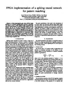
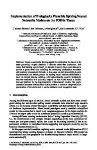
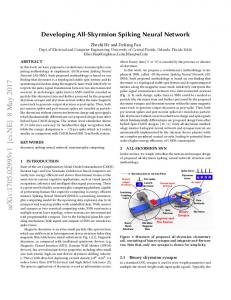
Figure 1.1: a) Schematic drawing of a neuron after Ramón y Cajal; dendrites, soma and axon can clearly be distinguished. Figure taken out of [Ger99]. b) Membrane potential V (t) (A) depending on presynaptic inputs (B). Many postsynaptic potentials (PSPs) are superimposed and eventually make V (t) cross the spiking threshold ϑ . In this case an action potential (which exceeds the scale of the plot) is fired. Afterwards V (t) runs through a phase of hyper-polarization. Figure adapted from [Brü04].

The synapses act as a preprocessor of the information arriving at a neuron’s dendrite in terms of modulating the effect on the postsynaptic neuron, which is located after the synapse. Modulating in this sense means weighting the presynaptic input in terms of its strength and also its sign. The term sign requires a closer look at the cell membrane of the neuron that divides the intracellular from the extracellular space and has a certain membrane capacitance Cm . Without any external input, the potentials on either side of the membrane differ and the resting potential Vrest is developed over Cm . It represents the steady state of concurring ion channels increasing, respectively decreasing, the membrane potential which is also called polarization in neuroscience. External input that increases the membrane potential is said to be depolarizing, the according synapse with a positive sign is excitatory. The contrary process is called hyper-polarization and the according synapse is inhibitory. The functionality of a neural system strongly depends on the configuration of its synapses. The possibility of dynamically changing the synapse weights is called plasticity. This change in the effect of a presynaptic signal on the postsynaptic neuron forms the basis of most models of learning and development of neural networks. Neurons communicate with action potentials, or spikes, which is illustrated in figure 1.1 b. Such a spike is a short (1 ms) and sudden increase in voltage that is created in the soma and travels down the axon. Reaching a synapse, the spike triggers a change in the synapse’s postsynaptic potential (PSP) which adds to the membrane voltage and then slowly decays with time. Several PSPs eventually rise the membrane voltage over a threshold ϑ . In this case, the neuron itself generates an action potential and after some time of hyper-polarization the membrane returns to the resting potential, if no further input is provided. As the spikes sent

1.2. THE UTILIZED INTEGRATE-AND-FIRE MODEL

7

out by one neuron always look the same, the transported information is solely coded within their firing times.

1.1.1

Modeling Biology

Modeling of neural systems can be classified into three generations as proposed by Maass in his review on networks of spiking neurons [Maa97]. These classes of models are distinguished according to their computational units and the term generations also implies the temporal sequence in which they have been developed. The first generation is based on the work of McCulloch and Pitts [MP43] who proposed the first neuron model in 1943. The McCulloch-Pitts neurons are a very simplified model of the biological neuron that accept an arbitrary number of binary inputs and have one binary output. Inputs may be excitatory or inhibitory and the connection to the neuron is also established by weighted synapses. If the sum over all inputs exceeds a certain threshold, the output becomes active. Many network models have their origin in McCulloch-Pitts neurons, such as multilayer perceptrons [MP69] (also called threshold circuits) or Hopfield nets [Hop82]. It was shown by McCulloch and Pitts that already the binary threshold model is universal for computations with digital input and output, and that every boolean function can be computed with these nets. The second generation of neuron models expands the output of the neuron in a way, that an activation function is applied to the weighted sum of the inputs. The activation function has a continuous set of possible output values, such as sigmoidal functions or piecewise linear functions. Past research work done within the Electronic Vision(s) group has focused on multilayer perceptron experiments that were performed on the basis of the HAGEN chip [SHMS04] developed within the group. See for example [Hoh05, Sch05, Sch06]. Both, first and second generation models work in a time discrete way. Their outputs are evaluated at a certain point in time and the temporal history of the inputs is neglected during this calculation. For an approximate biological interpretation of neural nets from the second generation, the continuous output values may be seen as a representation of the firing rate of a biological neuron. However, real neurons do code information within spatio-temporal patterns of spikes, or action potentials [Maa97]. Knowing this, a spike-based approach, which predicts the time of spike generation without exactly modeling the chemical processes on the cell membrane, is a viable approach to realize simulations of large neuron populations with high connectivity. The integrate-and-fire model [GK02] follows this approach and reflects the temporal behavior of biological neurons. The third generation of neuron models covers all kinds of spiking neural networks exhibiting the possibility of temporal coding. The analog VLSI implementation of a modified integrate-and-fire model will serve as a basis for the work described in this thesis. Note that a quantitative neuron model has been developed by Hodgkin and Huxley in 1952 [HH52]. This model uses a set of differential equations to model the current flowing on the membrane capacitance of a neuron. It has been shown by E. Mueller, that it is possible to fit the behavior of the integrate-and-fire model to that of the HodgkinHuxley model with regard to the timing of the generated action potentials [Mue03].

1.2

The Utilized Integrate-and-Fire Model

In this section, the selected model for the VLSI implementation is described. It is based on the standard integrate-and-fire model and allows the description of most cortical neuron types, while neglecting their spatial structure. The selection of the model is a conjoint work of E.

8


Mueller and Dr. J. Schemmel, whereas the analog implementation was carried out by Dr. J. Schemmel. The integration within the presented ASIC is one subject to this thesis. To be able to predict the requirements for the interfaces to the VLSI circuits as well as the the communicational needs in the entire system, the dynamics of the neural network are discussed after the model description.

1.2.1

Neuron and Synapse Model

The chosen model, in accordance to the standard integrate-and-fire model, describes the neuron’s soma as a membrane with capacitance Cm in a way that a linear correspondence exists between the biological and the model membrane potential V . If the membrane voltages reaches a threshold voltage Vth , a spike is generated, just as in the case of the biological neuron. The following effect of hyper-polarization is modeled by setting the membrane potential to the reset potential Vreset for a short time, e.g. the refractory period, where the neuron does not accept further synaptic input. The simple threshold-firing mechanism of the integrate-andfire model is not adequate to reflect the near-threshold behavior of the membrane. The very near-threshold behavior has been observed in nature [DRP03]. Therefore, the circuit has been designed such that the firing mechanism not only depends on the membrane voltage, but also on its derivative. In biology, spikes are generated by ion channels coupling to the axon. In contrast to this, the VLSI model contains an electronic circuit monitoring the membrane voltage and triggering the spike generation. To facilitate communication between the neurons, the spike is transported as a digital pulse. As it will be described in the following section, these pulses are either directly connected to other neurons on the same die which preserves the time continuous, asynchronous operation of the network. Furthermore, the time of spike generation may be digitized and the spike may be transported using synchronous digital communication techniques. Regardless of the underlying communication, the digitized neuron outputs are connected to the membrane of other neurons by conductance based synapses. Upon arrival of such a digital spike, the synaptic conductance follows a time course with an exponential onset and decay. Within the selected model, the membrane voltage V writes Cm

dV = gleak (V − El ) + ∑ p j (t) g j (t) (V − Ex ) + ∑ pk (t) gk (t) (V − Ei ) . dt j k

(1.1)

The constant Cm represents the total membrane capacitance. Thus the current flowing on the membrane is modeled multiplying the derivative of the membrane voltage V with Cm . The conductance gleak models the ion channels that pull the membrane voltage towards the leakage reversal potential1 El . The membrane finally will reach this potential, if no other input is present. Excitatory and inhibitory ion channels are modeled by synapses connected to the excitatory and the inhibitory reversal potentials Ex and Ei respectively. By summing over j, all excitatory synapses are covered by the first sum. The index k runs over all inhibitory synapses in the second sum. The time course of the synaptic conductances is controlled by the parameters p j,k (t). To facilitate the investigation of the temporal development of the neural network model, two plasticity mechanisms are included in the synaptic conductances g j,k (t), which are modeled by g j,k (t) = ω j,k (t) · gmax (1.2) j,k (t) , 1 The

reversal potential of a particular ion is the membrane voltage at which there is no net flow of ions from one side of the membrane to the other. The membrane voltage is pulled towards this potential if the according ion channel becomes active.


9

with the relative synaptic weight ω j,k (t) and a maximum conductance of gmax j,k (t). Developmental changes (like learning) within the brain, or generally within a neural network, are described by plasticity mechanisms within the neurons and synapses. The herein described model includes two mechanisms of synaptic plasticity: STDP and short term synaptic depression and facilitation. The actual implementation of these models has already been published in [SGMM06] and [SBMO07]. To motivate the need for precise temporal processing of neural events the STDP mechanism will be described in the following. Spike Timing Dependent Plasticity (STDP) Long term synaptic plasticity is modeled by an implementation of STDP within each synapse. It is based on the biological mechanism as described in [BP97, SMA00]. Synaptic plasticity is herein realized in a way that each synapse measures the time difference ∆t between preand postsynaptic spikes. If ∆t < 0, a causal correlation is measured (i.e. the presynaptic signal contributed to an output spike of the according neuron) and the synaptic weight is increased depending on a modification function. For acausal correlations the synaptic weight is decreased. The change of the synaptic weight for each pre- or postsynaptic signal is expressed by a factor 1 + F(∆t). F is called the STDP modification function and represents the exponentially weighted time difference ∆t. It is defined as follows: ( A+ exp( τ∆t+ ) if ∆t < 0 (causal) F(∆t) = (1.3) −A− exp(− τ∆t− ) if ∆t > 0 (acausal)

1.2.2

Terminology

Two terms regarding neural activity, which will be used throughout the thesis, shall be defined in this section: spike train and firing rate Spike Train According to the definition in [DA01] action potentials are typically treated as identical stereotyped events or spikes, although they can vary somewhat in duration, amplitude, and shape. Ignoring the brief duration of an action potential (about 1 ms), a sequence of action potentials can be characterized simply by a list of the times when spikes occurred. Therefore, the spike train of a neuron i is fully characterized by the set of firing times (1)

(n)

Fi = {ti , ...,ti }

(1.4)

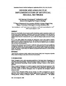
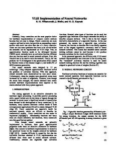
(n)

where ti is the most recent spike of neuron i. Figure 1.2 illustrates the activity recorded (the spike trains) from 30 arbitrarily selected neurons within the visual cortex of a monkey. Firing Rate Considering the large number of neurons in the brain it is nearly impossible to evaluate every single spike with respect to its exact timing. On this account, it has traditionally been thought that most, if not all, of the relevant information was contained in the mean firing rate of the neuron which is usually defined as a temporal average. Within a time window T = 100 ms or

10


Figure 1.2: Spatio-temporal pulse pattern. The spikes of 30 neurons (A1-E6, plotted along the vertical axes) out of the visual cortex of a monkey are shown as a function of time (horizontal axis, total time is 4 seconds). The firing times are marked by short vertical bars. The grey area marks a time window of 150 ms. Within this time, humans are able to perform complex information processing tasks, like face recognition. Figure taken from Krüger and Aiple [KA88].

T = 500 ms the number of occurring spikes nsp (T ) is counted. Division by the length of the time window gives the mean firing rate f=

nsp (T ) T

(1.5)

in units of s−1 or Hz. More definitions of firing rates can be found in [DA01], where the firing rate is approximated by different procedures, e.g. by using a Gaussian sliding window function. To evaluate the performance of the event processing techniques introduced within this thesis, the definition in equation 1.5 will be used. Note that it cannot be all about firing rates. The boxed grey area in figure 1.2 denotes T = 150 ms and obviously no mean firing rate can be given for this time window. Nevertheless is the brain capable of performing tasks like face recognition already within this time span. Consequently, the spatio-temporal correlation of the single spikes has to be considered when modeling a nervous system. While this is fulfilled by fact for the integrate-and-fire model itself, it is important to keep in mind that the underlying event transport mechanisms need to provide transport latencies that preserve the latencies introduced by biological synaptic connections.

1.2.3

Expected Neural Network Dynamics

The aim to model biological neural systems with dedicated hardware on the one hand requires the selection of a specific model which has been described in the preceding section. On the


11

other hand, the communication of neural events within the system has to be considered. In the selected model spikes are communicated as digital pulses between the neurons. The development of appropriate communication channels requires the knowledge of spike rates that are to be expected and other temporal constraints that arise from the topology of the biological system. Three items are selected to serve as basic constraints for the work presented within this thesis. Regarding spike rates neurons being in a high-conductance state and synchronized behavior of neural networks are selected to account for average and peak spike rates. Furthermore, connection delays observed in nature are taken as a minimum delay constraint for the different communication channels. The High-Conductance State The term high-conductance state describes a particular state of neurons within an active network, as typically seen in vivo, such as for example in awake and attentive animals. A single neuron is said to be in the high conductance state, if the total synaptic conductance received by the neuron is larger than its leakage conductance. First in vivo measurements proving the existence of the high-conductance state have been performed by Woody et al. [WG78]. In a review paper by Destexhe et al. [DRP03] the mean firing rate fhc of a neuron being in the high conductance state is found to be: 5 Hz < fhc < 40 Hz .

(1.6)

Synchronized Behavior Synchronized behavior is used in this context to describe the coherent spike generation of a set of neurons. Periodic synchronization has been observed within simulations by E. Mueller [MMS04] at a rate of 5 − 7 Hz within a network of 729 neurons. Stable propagation of synchronized spiking has been demonstrated by Diesmann et al. also by means of software simulations [DGA99]. To estimate the consequences of this behavior on the transport of the digitized events within a digital network (cf. chapter 3), the synchronized behavior is modeled within this thesis using a rate-based approach2 . For a set of neurons, an average firing rate fav is assumed for the time toff in between the synchronized spikes and a firing rate of fpeak during synchronized spiking, which lasts for ton . The values for fpeak and ton will be chosen in a way that the neuron generates at least one spike within ton . Connection Delays The connection delay between two biological neurons comprises the signal propagation delay along the axon of the neuron and the delay through the synapse with the subsequently connected dendrite. Depending on the spatial structure of a neural network, the delay between different neurons varies with their relative distance. A physical model that is based on analog VLSI circuits and the transport of digitized events, exhibits the same behavior and its delay should be tunable to reflect the biological values. Specific delay values strongly depend on the spatial structure of the simulated network, i.e. the benchmark for the hardware model. On the one hand, minimum delay values for synaptic transmission of 1–2.5 ms have for example been observed during in vitro measurements of the rat’s cortex by Schubert et al. [SKZ+ 03]. On the other hand, during software simulations 2 Spikes are generated with a probability p at a point in time. p is the average firing rate per unit time. Spike generation is uncorrelated to previous spikes (intervals are poisson distributed).

12


commonly used delay values are in the range of 0.1–1.5 ms for networks with a size of approximately 103 neurons [Mul06]. As a consequence of these figures, it can be said that hardware simulated delays should continuously cover possible delay values from approximately 0.1 ms upwards. Considering a speed-up factor of 105 for the hardware, this yields a minimum delay requirement of approximately 1 ns.

1.3

VLSI Implementation

We will now have a closer look at the actual implementation of the network model in analog VLSI hardware. It has already been stated in the previous section that parts of the circuits have already been published. However, a concise description of the whole model and especially of the neuron and synapse circuits is in preparation by Dr. J. Schemmel et al. and will therefore be omitted here. The following qualitative description is intended to give an outline of what served as a basis for the concepts developed, and the ASIC design that has been done throughout this thesis work.

1.3.1

Neuron Functionality

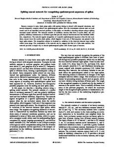
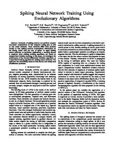
The operating principle of the neuron and synapse circuits is shown in figure 1.3. Circuits for synaptic short term plasticity are located within the synapse drivers and are omitted for simplicity. The circuits implementing STDP are located within each synapse and implement equation 1.3 all in parallel. They are also omitted for reasons of simplicity. The circuit topology is an array of synapses where every column of synapses connects to one neuron circuit. Each neuron circuit contains a capacitance Cm that physically represents the cell membrane capacitance. Three conductances model the ion channels represented by the three summands in equation 1.1. The reversal potentials El , Ex and Ei are modeled by voltages that are common for groups of several neurons each. This is the same for the threshold and the reset voltages Vth and Vreset . The membrane leakage current is controlled by gleak which can be set for each neuron. spike in

Vout

Vin

Iout excitatory

Vmax e/i

trise tfall

Iout

inhibitory

Vin

synaptic weight ram

4-input mux

synapse driver

Iin

spike out

synapse neuron

xi

Vth El Ex Ei gleak gx(Ix) gi(Ii)

Cm

Vreset

Figure 1.3: Block diagram of the neuron and synapse functionality in the analog VLSI implementation. Figure taken out of [SGMM06].

1.3. VLSI IMPLEMENTATION

13

In biological systems the synapse conductances are controlled by a chemical process within each synapse. In contrast to this, the analog VLSI implementation follows a different approach: the synapses produce a current output and the conductances are separately controlled for all excitatory and all inhibitory synapses at once. Two conductances, gx (Ix ) for the excitatory and gi (Ii ) for the inhibitory synapses, are located within the neuron. Thereby the current generated by the active synapses within the array is summed to an excitatory sum Ix and an inhibitory sum Ii . Two wires exist in each column to collect these current sums. The type of synapse can be set row wise and the synapses of one row all add their output current to the same wire. The spike generation process is triggered by a comparator that compares the membrane voltage with the threshold voltage. If a spike is generated, the membrane is pulled to the reset potential for a short period of time which hyper-polarizes the membrane in accordance with the integrate-and-fire model. In contrast to biology, the axon of the neuron is electrically isolated from the membrane and carries a digital pulse after the spike has been generated. The comparator is tuned in a way that its dependency on the derivative of the membrane voltage makes its behavior resemble that of the Hodgkin-Huxley model [SMM04].

1.3.2

Synapse Functionality and Connectivity

Due to the array structure, the number of synapses determines the area demand of the VLSI implementation. The size of a single synapse is therefore kept small by relocating some of its functionality into the row drivers that are placed at the left edge of the array, as illustrated in figure 1.3. As a result, the presynaptic signal is common for one synapse row and all associated neurons simultaneously receive the postsynaptic signals generated by the different synapses. The connectivity inside the array is illustrated in figure 1.4: presynaptic signals are shown as dotted lines and are horizontally routed through the array. Synapses are drawn as spheres and connect the presynaptic signal to the postsynaptic signal within each column. The postsynaptic signals use dashed arrows and are vertically routed to the neuron below. Only one of the two wires for Ix and Ii is displayed for simplicity. 125

126

synapse drivers

column#

127

post-synaptic signals to neurons pre-synaptic signals from synapse drivers neuron outputs to synapses and synapse drivers

neurons

Figure 1.4: Connection scheme used within the synapse array. A cutout of rows 125 to 127 is shown, which have been selected arbitrarily. Figure adapted from [SMM04].

The axon of the neuron is routed back into the array. On the one hand this allows the STDP circuits within the synapses to measure the time distance between the presynaptic and the postsynaptic signal. On the other hand, a horizontal line in each row connects the neuron with the corresponding number (the connection points are set on the diagonal of the array) to the

14


synapse driver at the edge. The input to the synapse driver can be selected out of this signal or three different external sources which is denoted by the 4-input multiplexer in figure 1.3. Further details regarding this connectivity will be given in section 4.2.2. The synapse driver converts a digital spike to a triangular voltage slope with adjustable rise and fall time and adjustable peak voltage. This ramp is converted to a current slope with exponential onset and decay by a current sink within each synapse. The current sink consists of 15 n-type metal oxide semiconductor (NMOS) transistors and the overall strength of the synaptic current is controlled by a 4 bit static weight memory within each synapse. Depending on the stored weight, the according number of transistors are activated and add to the synaptic current. As a result, the synaptic weight can be set with a resolution of 4 bit. A control line connected to the synapse driver sets the complete row to add its current to the excitatory or the inhibitory line. The storage of the synaptic weight within a digital memory requires a larger area than capacitance based solutions which have been used within a previous ASICs developed within the Electronic Vision(s) group [SMS01, SHMS04]. Digital weight storage within each synapse has still been chosen for two reasons: • The need for a periodic refresh of the capacitively stored weight introduces a significant communication overhead over the external interface of the chip. • The implementation of STDP within the chip requires the modification of the synaptic weights depending on their current value. Weights that have been modified by the STDP algorithm cannot be reflected by an external memory without transmitting the modified weight off chip.

1.3.3

Operating Speed and Power Consumption

Operating Speed of the Model The analog VLSI model aims to complement software simulations and digital model implementations. To justify this demand, the realization in silicon is designed such that it makes good use of the available resources in terms of area and speed. Many of the implemented silicon devices (transistors, capacitors, etc.) are close to the minimum size geometry. As a result, almost 100,000 synapses and 384 neurons fit on one die (cf. section 4.2). The small size results in low parasitic capacitance and low power consumption. Furthermore, the scaling of capacitances, conductances and currents leads to time constants in the physical model which lead to a speed-up factor of 105 for the model time compared to biological real time, i.e. 10 ns of model time would equal 1 ms in real time. The possibility to adjust parameters like rise and fall time of the synaptic current, membrane leakage current and the threshold comparator speed allow for a scaling of this factor within one order of magnitude resulting in a speed-up of 104 to 105 . Power Consumption According to [SMM04] the static power consumption of one neuron is about 10 µW. It is mainly caused by the constantly flowing bias currents and the membrane leakage. This low power density demonstrates the advantage of a physical model implementation compared to the usage of standard microprocessor for digital simulations. The power dissipation even of large chips with 106 neurons will only reach a few Watts. No definite value for the overall power consumption of the spiking neural network model can be given, because the synapse circuits do only consume power during spike generation. However, a good approximation of the maximum power consumption is to calculate the dynamic power consumption of the maximum number of synapses that may be active, simultane-


15

ously at an average firing rate which reflects the maximum expected rate. A rough estimation will be given in section 4.4.3.

1.3.4

Network Model and Potential Topologies

The network model is based on the transport of digital spikes from one neuron to multiple destination neurons reflecting the fan out of the axon of the biological neuron to the dendrite trees of several destination neurons. Thanks to the digital nature of the spike, the transmission may take place over large physical distances, also to neurons located on different chips. One possibility to transmit digital neural events is to use an address event representation (AER) protocol. An address defining the neuron is asynchronously transmitted together with an enable signal within this protocol which is for example used in VLSI spiking neural networks that operate in real time developed by Douglas et al. [OWLD05, SGOL+ 06]. Problems arise for the presented model due to the asynchronous nature of this protocol: if an accuracy of less than 0.1 ms biological real time is desired for the spike transmission, a maximum skew of about 1 ns on an AER bus would be required which is not feasible within large VLSI arrays or between several chips. For this reason, events that are to be transported off chip leave the continuous time domain and are digitized in time. The digitization process is described in the following section which also gives an overview of the overall analog VLSI implementation. The following network topologies can be realized with this model: in principle, a digitally generated spike can be duplicated any number of times and then be distributed to the synapse drivers located on several chips. Each synapse driver provides the fan out of its associated synapse row. Neglecting the signal propagation delay within the row, the axonal connection delay is the same for all target neurons within one row. One of the two goals of the presented thesis is the development of a communication protocol and the according hardware which together enable this event transport between different chips. This concept will be described in chapter 3.

1.3.5

Overview of the Implementation

A block diagram of the VLSI implementation of the physical model is shown in figure 1.5. The central synapse array is organized in two blocks, each containing 192 × 256 synapses. Each synapse consists of its four bit weight memory, the according digital-to-analog converter (DAC) and the current sink that produces the desired output slope. Furthermore, each synapse contains circuits measuring temporal correlations between pre- and postsynaptic signal, that are used for long term synaptic plasticity, e.g. STDP. Synapse control circuitry and the correlation readout electronics have digital interfaces that are part of an internal data bus that is connected to synchronous digital control logic. The process of spike generation within the neuron has already been described in the preceding sections. Digital spikes generated by the neurons are not only fed back to the synapse drivers but are also digitized in time to be transported off chip. The digitization happens with respect to a clock signal and involves several steps: the spiking neuron is identified by an asynchronous priority encoder that transmits the number (address) of the neuron to the next stage. If more than one neuron fires within one clock cycle, the one with the highest priority3 is selected and transmitted within that cycle. In the following cycle, the number of the next neuron is transmitted and so on. 3 The

priority is determined by the address of the neuron. Lower address means higher priority.

10 Bit DAC

output buffers


digital-to-time conv.

correlation measurement

right synapse drivers

DAC controlled conductance

post-pre

2 x 192 x 256 synapses weight RAM

pre-post

left synapse drivers

synapse ram control

48 to 1 mux

384 membrane voltage buffers

correlation readout


2967 bias current memories and 64 bias voltage generators

16

384 neurons

asynchronous priority encoder DLL time-to-digital converter synchronous digitaldigital part control

external interface

Figure 1.5: Block diagram of the analog VLSI implementation of the physical model. Figure adapted from [SMM04].

Two actions are carried out by the time to digital converter (TDC): on the one hand, it registers the number of the selected neuron to synchronize it to the clock signal. The stored value is the first part of the digitized event’s data, the address. On the other hand, the TDC measures the point in time of the spike onset. This is done by means of a delay-locked loop (DLL) dividing one clock cycle into 16 equally spaced time bins. If two neurons fire within one clock cycle, the second spike will thus have a maximum error of one clock period. In addition to the time bin information, a system time counter synchronous to the digitization clock is required. Its value during the digitization process completes the time stamp of the event and thus the event data. Digitized events are forwarded by digital control logic to be sent off the chip. The process of external event generation is initiated by sending an event to the digital control logic. The event data consequently consists of an input synapse address and a time stamp which itself consists of the system time and the time bin information. The digital control logic delivers the event within the desired system time clock cycle to the spike reconstruction circuits. These contain an address decoder and a digital to time converter (DTC), which operates based on the same DLL as the TDC. A digital pulse is generated at the input of the addressed synapse driver within the according time bin. To account for the high speed-up factor of the model, the event generation and digitization circuits are designed to operate at clock frequencies of up to 400 MHz. Thus, the precision of


17

the time measurement theoretically will reach at best 156 ps which equals 1/16 of the clock period. In biological time, this results in an accuracy of 15.6 µs. No two biological neurons or synapses are alike. Different surroundings, different physical size and connectivity lead to varying properties like the membrane capacitance, the leakage currents or differences in the synaptic behavior. The implementation of the model by means of analog VLSI has similar implications: no two transistors or generally no two analog devices are alike. While this deems desirable, it should still be possible to tune model parameters as to mimic a specific behavior and furthermore to eliminate drastic differences which may occur due to mismatching of two circuits. The behavior of analog circuits can be tuned by means of bias voltages or currents or other parameter voltages. This is done by a DAC that connects to different current memory cells and parameter voltage generators storing parameters like the leakage conductance or the reversal potentials. A more precise description of the parameter generation will be given in chapter 4 and a complete list of parameters can be found in appendix C.

18


Chapter 2

System on Chip Design Methodology

The implementation of full custom analog electronics in contrast to the design of digital ASICs is commonly carried out using different design methodologies. The key aspect covered within this thesis is the implementation of analog VLSI circuits comprising several millions of transistors together with highspeed digital logic into one mixed-signal ASIC by the usage of a customized, automated design flow. This chapter describes this design flow, whereas the actual implementation and the properties of the ASIC are covered in chapter 4. The necessary data preparation needed for the logical synthesis and the physical integration is described followed by a general outline of the logical synthesis process. For the physical implementation, Cadence First Encounter is used and besides the common implementation process, developed strategies for the system integration and the implementation of high speed digital interfaces are described. As a result, the analog electronics introduced in chapter 1 are seamlessly integratable together with the digital logic detailed in the following chapters. The verification process, including timing closure and physical verification, closes the chapter.

Generally, the process of designing an ASIC can be divided into two phases called the front end which is the starting point of the design process, and the back end where the physical implementation is carried out. Concerning digital logic, the front end design starts with a behavioral description of the ASIC using a high-level hardware description language, such as Verilog or VHDL4 . The following digital circuit synthesis involves the translation of the behavioral description of a circuit into a gate-level netlist comprising generic logic gates and storage elements. For the physical implementation, these generic elements need to be mapped to a target technology. This technology consists of a library of standard logic cells (AND, OR, etc.) and storage elements (flip-flops, latches) that have been designed for a specific fabrication process. This mapped gate-level netlist serves as a starting point for the digital back end. 4 Very

High Speed Integrated Circuit Hardware Description Language.

19

20

CHAPTER 2. SYSTEM ON CHIP DESIGN METHODOLOGY

Within a purely analog design process, the front end consists of the initial schematic5 capture of the circuit. It is tuned and optimized towards its specifications by means of analog simulations. The final schematic subsequently serves as a basis for the physical implementation using the back end. The back end in general involves the physical implementation of the circuit, be it analog or digital. It consists of an initial placement of all components followed by the routing of power and signal wires. The mixed-signal design process described within this chapter allows for the automated integration of complete analog blocks into one ASIC together with digital logic in the back end process. Different, commonly rather generic design flows for purely digital and even mixed-signal ASICs are available through the online documentation of the design software vendor [Cad06b] or are available in text books (see for example [Bha99]). However, the implementation of large mixed-signal ASIC or system on chip (SoC)6 requires the development of non-standard solutions throughout a design flow, due to the special demands that arise from the (in many cases) proprietary interfaces and block implementations. The novel aspect of the presented flow is the automatic integration of complete, fully analog VLSI designs together with high speed digital logic into one ASIC. To integrate both analog and digital circuits, the following approach is used: The analog circuits are divided into functional blocks (later referred to as analog blocks) that together form the analog part of the chip. A top-level schematic for the analog part is drawn which interconnects these blocks and contains ports for signals needed for digital communication or off-chip connections. The developed scripts enable the digital back end software to import this analog top-level schematic together with the digital synthesis results. By partitioning the design into an analog and a digital part, each part is separately physically implemented using different sets of rules. The final chip assembly which involves the interconnection of analog and digital part, connections to bond pads, final checks and the functional verification finishes the design. It is done together for both, analog and digital circuitry, by a common set of tools. The design flow is illustrated in figure 2.1 as an initial reference. In the following section, some prerequisites are introduced to clarify the terminology used throughout this chapter. The subsequent description of the design flow will intermittently refer to figure 2.1.

2.1

Prerequisites

Two very basic concepts of digital design are explained to clarify the strategies described later on. Following this, the data necessary for the implementation of hierarchical blocks using an automated design flow is explained. While this data is commercially available for the digital design, the corresponding analog design data is generated by a set of scripts which have been developed throughout the presented work.

2.1.1

Digital Design Fundamentals

Static Timing Analysis The static timing analysis (STA) allows for the computation of the timing of a digital circuit without requiring simulation. Digital circuits are commonly characterized by the maximum clock frequency at which they operate which is commonly determined using STA. Moreover, delay calculations using STA are incorporated within numerous steps 5 Schematic

will be used as the short form of schematic diagram, the description of an electronic circuit. on chip design is an idea of integrating all components of an electronic system into a single chip. It may contain digital, analog and mixed-signal functions. 6 System

2.1. PREREQUISITES

21

analog front & back end full custom layout abstract

RTL Verilog

schematic

abstract

macro inst. Verilog

SPICE netlist

Simulation NCSIM

sim. model

timing lib

Synthesis Synopsys

timing constr.

synth_top.v

STA PrimeTime

Simulation NCSIM

STA PrimeTime

Simulation NCSIM

Place & Route First Encounter

pnr_top.v

GDSII

Cadence Virtuoso FE design flow GDSII

LVS

floorplan, create partitions DRC analog implementation

digital implementation

submission unpartition

Figure 2.1: Illustration of the developed design flow for the implementation of large mixed-signal ASICs. Solid arrows denote subsequent steps in the flow. Dashed arrows show dependencies on input data and constraints.

throughout the (SoC) design process, such as logic synthesis and the steps performed during physical implementation in the digital back end. The speed-up compared to a circuit simulation is due to the use of simplified delay models and the fact that its ability to consider the effects of logical interactions between signals is limited [Bha99]. In a synchronous digital system data is stored in flip-flops or latches. The outputs of these storage elements are connected to inputs of other storage elements directly or through combinational logic (see figure 2.2). Data advances on each tick7 of the clock and in this system two types of violations are possible: a setup violation due to the signal arriving too late to be captured within the setup time tSU before the clock edge. Or a hold violation due to the signal changing before the hold time tHD after the clock edge has elapsed. The following terms are used throughout the design flow in conjunction with STA: 7 The

flip-flops may be triggered with the rising, the falling or both edges of the clock signal.

22


D1

clk

Q

D C

Q1

combinational logic

D2

Q

D

Q2

C

Figure 2.2: Illustration of a synchronous digital system. Ideally, the clock signal clk arrives simultaneously, data is delayed by the clock to output time Tco and the delay through the combinational logic.

• The critical path is defined as the path between an input and an output with the maximum delay. It limits the operating frequency of a digital circuit. • The arrival time is the time it takes a signal to become valid at a certain point. As reference (time 0), the arrival of a clock signal is often used. • The required time is the latest time at which a signal can arrive without making the clock cycle longer than desired. • The slack associated with a path between two storage elements is the difference between the required time and the arrival time. A negative slack implies that the circuit will not work at the given clock frequency.

tSU tHD

clock signal

according data signals

data valid window

Figure 2.3: Timing specification for the source synchronous HyperTransport interface [Hyp06]. To maximize the data valid window, tSU and tHD are to be maximized.

Source Synchronous Data Transmission In contrast to synchronous digital systems, where one clock is distributed to all components of the system, in a source synchronous system a corresponding clock signal is transmitted along with the data signals. Source synchronous data transmission is commonly used for high-speed physical interfaces such as the HyperTransport interface [Hyp06] or the double data rate SDRAM (DDR-SDRAM) interface [Mic02]. Source synchronous interfaces are point-to-point connections where only the relative timing of the clock signal and the corresponding data signals need to be specified. One advantage is that these signals may be routed throughout the system with equal delay and no care has to be taken about the clock distribution to other parts of the system as in synchronous systems. Moreover, the circuits generating clock and data signals are located on one die. As a consequence, delay

2.1. PREREQUISITES

23

experienced by the data through a device tracks the delay experienced by the clock through that same device over process variations. Figure 2.3 illustrates the timing specified for the HyperTransport physical interface which is implemented in the presented chip.

2.1.2

Required Technology Data

The technology data needed for the integration of analog blocks using the digital back end is described in this section. The Standard Cell Library The standard cell library consists of a set of standard logic elements and storage elements designed for a specific fabrication process. The library usually contains multiple implementations of the same element, differing in area and speed, which allows the implementation tools to optimize a design in either direction. Basis for each standard cell is an analog transistor circuit and the corresponding layout. To make use of this cell for a digital design flow, it is characterized regarding its temporal behavior on the pin level and its physical dimensions. A behavioral simulation model written in a hardware description language (HDL), the timing information and the physical dimensions are stored within separate files that together define the standard cell library. The integration of analog blocks as macro cells that are to be placed and routed using primarily digital back end tools requires the availability of this very data. The Technology Library A technology library describing standard cells contains four types of information (the format introduced by Synopsys is used and a complete description of the technology library format is given in [Syn04b]): • Structural information. Describes the connectivity of each cell to the outside world, including cell, bus, and pin descriptions. • Timing information. Describes the parameters for pin-to-pin timing relationships and delay calculation for each cell in the library. This information ensures accurate STA and timing optimization of a design. • Functional information. Describes the logical function of every output pin depending on the cell’s inputs, so that the synthesis program can map the logic of a design to the actual ASIC technology. • Environmental information. Describes the manufacturing process, operating temperature, supply voltage variations, all of which directly affect the efficiency of every design. For the implementation of analog blocks only the structural information and the timing information are important. The environmental information is predefined by the vendor within the standard cell library and functional information is not required as the block is to be implemented as-is and no optimization is to be performed on it. Different delay models are available for the description of the timing. Two commonly used ones are the CMOS linear and the CMOS non-linear delay models. For cells with a straight forward functionality like standard cells there are tools available8 that automatically characterize the cells using methods described for example in [SH02]. If no automatic characterization 8 No such tools are available at the Kirchhoff Institute. One example is SiliconSmart from Magma. (http://www.magma-da.com)

24


a)

pin(clk400) { clock : true ; max_transition : 0.15 ; direction : input ; capacitance : 0.319 ; }

b)

PIN clk400 DIRECTION INPUT ; USE CLOCK ; PORT LAYER ME2 ; RECT 10.03 0.01 10.31 0.29 ; END END clk400

Figure 2.4: a) Description of a clock pin using the Synopsys Timing Library Format and the linear delay model. b) Geometric description of the same pin using LEF.

tool is available, the linear model should be used. Therein the delay through a cell or macro is calculated based on the transition time of the input signal, the delay through the cell without any specific load and the RC-delay at the corresponding output that results from the output resistance of the cell’s driver and the capacitive load [Syn04b]. The intrinsic cell delay as well as the output resistance can be obtained by means of analog simulations. Values obtained this way are then embedded as timing information into a technology library. Several technology libraries are usually made available to reflect the best, worst and typical fabrication process variations. Figure 2.4 a shows a very simple example for the definition of a clock pin using the linear delay model. The Abstract View The layout data of an analog block cannot directly be used by the digital back end. Therefore, for the physical implementation, an abstract view is generated which reduces the analog layout to a block cell like it is the case for the cells within the standard cell library. The abstract view provides information like the cell name or its boundary. Pin names, locations, metal layers, type and direction (in/out/inout) are included and besides the pins the locations of all metal tracks and vias in the layout are included as obstructions. The abstract view is generated in the Cadence analog environment using the Cadence Abstract Generator. It is then converted to a text file in library exchange format (LEF) which is being read by the digital back end. An example for the LEF syntax is shown in figure 2.4 b. Obviously this text file becomes very large if all metal geometry of an analog VLSI block completely would be included. Especially inside analog VLSI blocks this information is surplus. The amount of information is reduced by merging small geometries (in the order of magnitude of the minimum width) to few large obstructing geometries. Merging is done in two ways: • Use the resize option provided by the software. All geometry data is first being widened, closing small gaps and then shrunk, thereby leaving over only coarse geometries. • Many overlapping shapes exist after this process and to further reduce the amount of data, these shapes are automatically merged by scripting the Virtuoso layout environment. Pins are generated automatically within the abstract view at locations labeled accordingly within the layout. To support non-quadratic or rectilinear pin geometries, the developed scripts support so called shape pins9 that override the automatically extracted pin information. This is especially useful for the generation of multiple connections to large power grids or connections to heavily loaded signal pins requiring a wide metal routing. To ease pin access for the router, the pins are preferably to be placed near the cell boundary. 9 This

is a geometry that s natively supported by the layout tool.

25

68µm

5.04µm

2.2. DESIGN DATA PREPARATION

2.2µm

268µm

Figure 2.5: Layout view of a standard cell inverter compared to the layout of an analog block. The inverter is comparably easy to access by an automated router, because only one metal layer is occupied by its layout. In contrast, care has to be taken to retain this accessibility at the complex layout of the multi-metal layered analog block to keep the automatic integration feasible.

On its left side, figure 2.5 shows the standard cell implementation of an inverter compared to the layout of an exemplary selected analog block (it is the block containing both the DTCs and the TDCs). The standard cell is designed to occupy only one metal layer and to have end-toend rails for power connections at the top and the bottom side. Pins can easily be connected by an automatic router by directly connecting to one of the pins from the second metal layer. Five of the six metal layers available in the utilized United Microelectronics Corporation (UMC) fabrication process are available for routing. In contrast to this, the analog block has many pins distributed on different metal layers over the whole area. To still enable an automatic router to connect to these pins, it has to be ensured that they are accessible from at least one direction. The Technology LEF File The process details relevant to the digital back end are specified in this text file. Preferred routing directions are defined for the different metal layers within this file10 as well as minimum metal wire width and routing pitch, physical parameters like thickness and sheet resistance, slotting and antenna rules, and rules for the via generation among the layers. According to these rules, the router performs routing at minimum width and pitch. Analog nets that require wider spacing or wider metal, require the manual specification of non-default rules additional to the standard rules. These non-default rules at least include the redefinition of the routing width, the spacing and the via generation - for reasons of simplicity, the reader may refer to the LEF language reference for details [Cad05a].

2.2

Design Data Preparation

The following paragraphs will briefly describe the steps that are taken from data preparation to the final submission of the layout data to fabrication according to figure 2.1. Analog Design Data The analog design includes the schematic capture and the physical layout of the macro blocks using the Cadence Virtuoso and AMS Designer platform. Each block is designed by hand and a physical check including design rule check (DRC)11 and layout versus schematic (LVS)12 is performed. The blocks may comprise small building blocks 10 Routing

direction is either horizontal or vertical. The router tries to route wires in the preferred direction first and only routes short segments in the other direction. 11 Checks for geometric errors. 12 Verifies the matching between devices in the layout and the schematic.

26


as for example single neuron or synapse circuits. In the case of the presented chip, VLSI blocks are implemented that already contain the connections among these small building blocks. To integrate a whole set of analog blocks including their interconnections automatically, the library data and abstract view described in the preceding section and a Verilog netlist are required. This netlist is generated by the following steps: • Create a schematic of the whole analog part including block interconnections and required ports. • Create empty behavioral descriptions of the analog blocks including only port descriptions. These are needed for correct instantiation and are generated automatically. • Make use of the netlisting functionality provided by the Cadence AMS Designer suite and create a Verilog netlist only consisting of the block instances. This is done script based within the presented flow to avoid errors after design changes. Digital Design Data The digital design includes the RTL13 or behavioral description of the digital part of the chip. Above all it includes the very top-level of the hierarchical design that is to be implemented using the proposed SoC design methodology. This top-level module is a Verilog netlist with ports representing physical pins of the chip instantiating digital and analog top-level modules (of course, several are possible). No glue logic must be used at this level as it only defines the connectivity and no optimization by the digital front end or back end is performed. For top-level verification purposes, the top-level module may be integrated into different simulation testbenches, be it behavioral or RTL descriptions of the controller, and simulated using either Cadence NCSIM for mixed-signal simulations or Mentor Graphics ModelSim for solely digital simulations14 . If digital macros like memory arrays are present in the design, the according library data has to be available before proceeding with the flow.

2.3

Logic Synthesis and Digital Front End

The task of the digital front end is to transform the RTL or behavioral description of an ASIC into a gate-level netlist. This process is called synthesis. After the initial translation into a netlist consisting of generic logic functions and storage elements (compile phase), this netlist is then mapped to the target technology using the elements available in the standard cell library (mapping phase). The design is then optimized for area, speed and design rule violations like maximum transition time or maximum capacitance violations (optimization phase). Especially the timing optimization requires the definition of consistent constraints to the software tools. Synopsys Design Compiler is used for the digital front end within this flow [Syn04a]. The timing constraints are defined using the tool command language (TCL) syntax which is supported by all other software throughout the flow that requires the specification of timing constraints for the design. This ensures consistent STA results at every stage of the flow. The synthesis is divided into two major steps within the presented design flow. First, the digital part is synthesized and optimized to meet its timing requirements. The correct specification of the timing is crucial for the correct functionality of the synthesized netlist. The periods of all clock signals need to be specified, thereby defining the maximum delay between 13 Register 14 Analog

Transfer Level: coding style that describes registers using a hardware description language. blocks are treated as black boxes using only the empty modules in this case.

2.4. DIGITAL BACK END AND SYSTEM INTEGRATION

27

two clocked elements. Apart from these synchronous constraints, asynchronous paths have to be identified and constrained with minimum or maximum delay, whichever is appropriate. To avoid unnecessary optimizations, paths that do not underly any timing constraints are marked manually as well. In a second step, the digital netlist obtained in the first step is combined with the analog netlist to form the top-level netlist of the chip. Only interface signals between analog and digital modules are optimized during this step. The top-level netlist is evaluated for timing problems using Synopsys PrimeTime and a functional verification is performed using the simulation tools ModelsSim or NCSIM, depending on the setup of the testbench. The purpose of the verification at this stage of the flow is to identify faulty timing constraints that lead to incorrect implementations. The final implementation is subject to the digital back end.

2.4

Digital Back End and System Integration

For the digital back end and the system integration, Cadence SoC Encounter is used. This software provides a complete hierarchical design solution, including features like floorplanning and virtual prototyping, hierarchical partitioning and block placement, logic optimization, timing optimization, signal wire and power routing, geometry verification, connectivity and process antenna verification and the generation of stream data (GDSII15 ). During the phase called virtual prototyping, it is possible to estimate the design’s performance very quickly by means of a fast trial-route algorithm, a built in RC-extraction and delay calculation algorithm, and a built-in STA algorithm. As SoC Encounter can be run in batch mode, the whole back end flow has been set up using scripts that are executed from within a make file. Reports are written at each step of the flow and the design process is fully reproducible.

2.4.1

Design Import and Partitioning

Apart from the data that is supplied by the standard cell vendor like LEF data and technology libraries for I/O cells and standard cells, the following data has to be generated respectively specified and imported into First Encounter: • The synthesized gate-level netlist of the chip (output of digital front end). • Consistent LEF data for the standard cells, digital macros and the analog blocks as well as the according technology library information. Besides the LEF and technology data for the standard cells, the same data has to be available for I/O cells that are to be used for the pad connections of the chip. These cells are also supplied by the standard cell vendor. • A timing constraint file. The constraint file used by the digital front end is included by this file to ensure the usage of identical constraints. Moreover, constraints that only apply to the back end can be given here. • A capacitance table file which serves as a basis for the RC calculations. This file is comprised of metal-metal capacitances and resistances for various configurations which are stored within look-up tables (LUTs). This file has to be generated separately and can have different levels of accuracy (the lower the accuracy, the faster the calculation). 15 GDSII is a hierarchical file format to exchange 2D design data. It contains only geometry information for the physical layers of an ASIC and is used to transfer the design data to the foundry.

28


• An I/O assignment file which defines the positions of the I/O cells. If the pinout is not fixed prior to the design start, this file may be changed iteratively during the initial floorplanning stages. • A very initial floorplan specifying the coordinates of the die boundary, the I/O ring and the core area. • A list of power and ground net names that are globally valid for the design. Power routing can only be done for these nets. This list is very important as the imported Verilog netlist does not contain any power connections and the power connections for the analog blocks are later on performed using this list. The sum of this data is called the configuration for SoC Encounter. Floorplan Floorplanning involves the definition of placement regions for modules, defining boundaries for top-level modules that will serve as partition boundaries, and macro cell placement. In the presented flow, the macro cell placement is done semi-automatic by placing macro cells with relative coordinates. One example is given in the following code snippet where a set of macros no__ is placed relative to another, absolutely placed macro nb_0_ with a pitch of 100 µm in x-direction: placeInstance analog_chip/nb_0_ 381.4 1800 MY for {set i 0} {$i 1 neural network chips are attached to the daisy chain, the logic described in this subsection should be implemented in a parallel manner for each of them. n event packets are 33 These

time stamps are monitored by registers in the box “network chip FIFO event time stamps”. catch the case the most recently stored time stamp has also been corrected, the developed algorithm offers the option to increase expired time stamps within a certain margin. This can be done with the logic used for the regular correction with only marginal modifications. 34 To

56

CHAPTER 3. LARGE SCALE ARTIFICIAL NEURAL NETWORKS

then available, each with its own value for the smallest tev,norm . In this case, the packet with the overall smallest tev,norm is to be sent first. The time stamps of the events sent are finally marked as most recently sent to the according event_buffer_in module on the neural network chip.

3.3.3

Implementation Considerations

The implementation of the EventRouter is subject to future work and therefore—within the presented thesis—only the concept and recommendations for the final implementations are shown. In the first version, the EventRouter will presumably be implemented in the FPGA of the Nathan module whose resources have to be shared among the logic needed for the implementation of the logic modules comprising the whole system: the basic environment of the FPGA consists of a memory controller and an external control interface (see section 5.2.1). For the operation of large scale spiking neural networks, four additional components are required: the controller logic, the playback memory, the switch and the EventRouter. This section gives first recommendations on the HDL35 implementation of the EventRouter and based upon these, the resource consumption of the final design is calculated to have an estimate whether the design will fit into the FPGA or not. Concerning the whole system, the following points can already be predefined: • The maximum clock frequency for the MGTs is 156.25 MHz. This should also be chosen as the operating frequency for the controller and the neural network chip itself because asynchronous operation would introduce additional delay. • As described in section 3.1.3, a single neural event consists of at least 12 bit of timing information and 9 bit for the neuron/synapse address. As a result, two 16 bit switch time slots at a time are required to transmit one event and the resulting rate for the resulting event time slots within one switch period is 78.125 MHz. Recommendations for the Different Modules EventOutQueue The EventOutQueue module (cf. figure 3.10) has to provide three interfaces. For the incoming events this should be a direct connection to the registers located within the controller, where incoming events are stored for the first time. On the output side, an adaption to the data structure expected by the VHDL implementation of the switch will be necessary for two reasons: first, data is being exchanged between the two synchronous clock domains which differ by a factor of two in frequency. Second, the current time slot of the switch has to be evaluated and a decision has to be made whether the module is addressed within this time slot or not. Besides the interfaces needed for event communication, an interface for configuration purposes and for monitoring features is needed which connects to the global FPGA infrastructure (cf. section 5.2.1). As the virtual connection to which an EventOutQueue is assigned automatically defines the destination chip address and the axonal delay, these two values need only to be stored once inside the module. The mapping of a source neuron address to a destination synapse row address has to be stored within a LUT. The Block SelectRAM resources of the Virtex-II Pro FPGA [Xil02a] are ideally suited for this task when storing the value of the destination address at the Block SelectRAM memory address representing the source neuron. This look-up has 35 The EventRouter could be implemented using either Verilog or very high speed integrated circuit (VHSIC) hardware description language (VHDL) as a HDL.

3.3. NEURAL EVENT PROCESSOR FOR INTER-CHIP COMMUNICATION

Component Comparator a < b, 8 bit Subtractor, 2 bit Adder/Subtractor, 8 bit Adder, 12 bit Smallest out of 3, 8 bit Multiplexer 3-in-1, 21 bit FIFO 66 × 64, BRAMs Register for data path Memory for constants Total

# required 3 1 3 3 1 1 1 100 20

BRAMs – – – – – – 2 – 2 4

Flip-Flops – – – 60 – – 153 100 20 309

LUTs 32 40 40 60 30 21 78 – – 221

57

Slices 16 25 25 30 15 21 96 50 10 241

Table 3.3: Logic components needed for the implementation of EventOutQueue. The resource consumption has been either obtained by synthesizing exemplary VHDL code or is based on the information supplied by the Xilinx CORE Generator [Xil05c] for generic components like comparators.

to be done for up to three incoming events in parallel. One Block SelectRAM features two independent address ports, so three LUTs will consume two such modules. The calculation of the destination time is done based on the delay value stored globally for the EventOutQueue module and requires a 12 bit adder. Destination time and address are stored after calculation which requires another 21 registers. The calculation of the number of events currently stored within the FIFO memory requires one 2 bit subtracter, one adder with a width of max. 8 bit and an according comparator. The subsequent storage of the events could then be done in a FIFO memory based on two Block SelectRAMs that account for the data width of 66 bit which is needed to store up to three events in parallel. On the pop-interface of the FIFO memory suitable asynchronous logic is needed that determines the event with the smallest time stamp. A suggestion for the implementation of this circuitry is the Parallel Rank Computer described by Hirschl et al. in [HY04]. The event with the smallest time stamp is then multiplexed to the output by a 21 bit 3-to-1 multiplexer. Finally, equation 3.8 needs to be calculated and the event can then be sent. Along with the multiplexer logic, this requires one comparator, one adder and one subtracter. Based on these considerations, the required components and their estimated resource consumption are summarized in table 3.3.

EventInQueue This module basically acts as a FIFO memory. The depth of this FIFO may be relatively small as described in section 3.3.1. In particular it has been proven by simulations that depths over 16 entries are not required (data not shown). Knowing this, another feature of the Virtex-II Pro FPGA can be exploited: each LUT of the FPGA fabric may be configured as 16 bits of distributed SelectRAM+ which can be seen as memory resources equally distributed over the FPGA fabric. The implementation of FIFO memories using distributed SelectRAM+ resources is described by Xilinx, Inc. in [Gop05] and a customized version of this FIFO has exemplarily been synthesized for the purpose of resource estimation. The only arithmetics required within EventOutQueue is the calculation of the front event’s time stamp normed on its transmission latency in the daisy chain based on equation 3.9 which requires one 8 bit subtracter. As in the case of EventOutQueue, some glue logic to interface to the switch ports

58


is additionally needed. The required components and their estimated resource consumption are summarized in table 3.4. Component Adder/Subtractor, 8 bit FIFO 21 × 16, BSRAMs Register for data path Memory for constants Total

# required 1 1 45 20

BRAMs – – – – –

Flip-Flops – 34 45 20 99

LUTs 8 38 – – 46

Slices 5 20 23 10 58

Table 3.4: Logic components needed for the implementation of EventInQueue. The resource consumption has been either obtained by synthesizing exemplary VHDL code or is based on the information supplied by the Xilinx CORE Generator [Xil05c] for generic components like comparators.

EventPctGen In section 3.3.2 the structure of the event packet generation logic (EventPctGen) has been described (see also figure 3.12). As indicated there, the actual implementation strongly depends on the number of virtual connections terminating at this module. If this number exceeds the number of events that can be packed into one data packet for the network chip, the EventInQueue modules are clustered at the single packet slots. Pipelining is necessary and in the first cycle, the EventInQueue containing the event with the smallest time stamp for delivery has to be determined. Resource consumption is estimated using the Parallel Rank Computer that has been used to select an event out of EventOutQueue in section 3.3.3. After this comparison, the three selected events are stored within three 21 bit pipeline registers. The next step involves the comparison of the time stamps of the selected events with the time stamps of the events that have most recently been stored in the event_buffer_in modules on the neural network chip. In figure 3.12 it is indicated, that this requires one 8 bit comparator and one 8 bit adder for each event slot in the data packet. The elements used for the storage of the time stamps within the event_buffer_ins depend on the timing margin left during implementation. Regarding timing (e.g. positive slack), the most promising approach would be an implementation using flip-flops but this requires # event_buffer_ins · width = 16 · 8 = 128 registers per neural network chip. If timing is not an issue, an implementation using Block SelectRAM or Distributed SelectRAM would be most resource efficient. VHDL code implementing the event packing algorithm described in section 3.3.2 has been written and synthesized to estimate the resource consumption of the afore described logic as well as the logic needed for the selection of the event with the smallest time stamp. Depending on the timing margin that results from the implementation, it might become necessary to introduce another pipeline stage between the existing pipeline registers and the registers for the final event packet. To have a conservative estimate, this is considered in the resource consumption of the module. Simulation results are not supposed to change due to this pipeline stage, since it only increases the minimum transmission latency that can be achieved on one virtual connection and has no influence on the other stages of the event processing. Table 3.5 summarizes all these components including the additional pipeline stage and the 128 additional registers. The numbers are calculated for three EventInQueues connected to the module. This module needs to be adapted to the existing FPGA modules at two points. Data sent by the playback memory and the event packets generated herein need to be merged. This integration can be done seamlessly as the output data path of the controller is already implemented in a way that prioritizes event packets (see section 5.2.3). Therefore, event processing should be

3.3. NEURAL EVENT PROCESSOR FOR INTER-CHIP COMMUNICATION

Component Comparator a < b, 8 bit Adder/Subtractor, 8 bit Smallest out of 3, 8 bit Multiplexer 3-in-1, 21 bit Fits-in-Packet logic Register for time stamp storage Register 2 × pipeline Register for event packet Memory for constants Total

# required 3 3 1 1 3 128 132 70 64

BRAMs – – – – – (3) – – – –

Flip-Flops – – – – – 128 132 70 64 394

LUTs 24 24 30 21 57 – – – – 156

59

Slices 12 15 15 21 33 64 66 35 32 293

Table 3.5: Logic components needed for the implementation of EventPctGen. The resource consumption has been either obtained by synthesizing exemplary VHDL code or is based on the information supplied by the Xilinx CORE Generator [Xil05c] for generic components like comparators.

disabled during the initialization and configuration phase of the chip to make sure all data are completely transmitted. Background Activity for the Neural Network As described in chapter 1 the simulation of neural networks either in software or in hardware will always be restricted to a very small fraction of the biological system. Thus, to develop a most realistic scenario, it is important to stimulate the set of simulated neurons with some sort of background activity that mimics the context of the biological network for the modeled neural network. In particular, this is required to induce the high-conductance state of the simulated neurons [DRP03, MMS04]. This background activity is provided locally on each Nathan module by events that are generated by the playback memory. This concept is also being used to provide the entire input for single-chip experiments with the presented chip by D. Brüderle [Brü07] and can easily be implemented together with the EventRouter logic. The respective outputs of the playback memory are connected to a corresponding EventInQueue within the EventRouter as shown in figure 3.7. Events providing the background activity are then sent by the playback memory in a way that their timing is equal to the timing of the incoming event streams. To accomplish this, the algorithm to generate the playback memory program (see section 5.3) needs to be modified in a way that it does not use the earliest possible point in time to transmit an event, but rather the latest possible point in time. Doing so, the events supplied by the playback memory will have similar time stamps as the ones coming from the switch.

3.3.4

Estimated Resource Consumption

An exact estimation of the resource consumption of the final design is not possible. Several factors need to be considered for a rough estimation: to begin with, the estimations given above only consider the components that are supposed to consume the most resources and neglect the functionality required for the integration into the existing logic framework. It is also not predictable to what extent the routing will consume resources. For reason of these considerations it has been decided to include a certain overhead into the calculations. Only a small error is expected for the number of needed flip-flops, the overhead is set to 20 %. The

60


overhead for LUT and slice utilization is set to a conservative value of 40 % as these values are harder to predict. Table 3.6 lists the resource consumptions including the overhead for the EventRouter. The values for the controller are taken from the final mapping report and correspond to the complete design including the external interface and the memory controller. The values for the switch represent a complete design including the synchronization logic with two switch ports to the MGT network and two to the EventRouter36 . No overhead has been calculated for the usage of Block SelectRAMs. Component EventRouter Controller Switch Total Available Util. EventRouter Util. Total

BRAMs 11 22 0 44 25.0% 75.0%

Flip-Flops 1571 3451 319 9856 15.9% 54.2%

LUTs 1064 3911 768 9856 10.8% 58.3%

Slices 1345 3203 500 4928 27.3% 102.4%

Table 3.6: Compilation of the resource consumption of the switch, the controller and the estimated overall resource consumption of the module EventRouter including an overhead. The numbers are calculated relative to the resources of the Virtex-II Pro FPGA XC2VP7 that is being used on the Nathan module [Xil02a].

The most reliable numbers in this calculation are the numbers of registers that will be used by the final design because it became obvious in the preceding sections how many data will have to be stored within one clock cycle. Logic functions that need to be implemented have been pre-synthesized and the calculated numbers include a conservative overhead. The final value for the occupied slice resources does not only depend on the logic functions to be implemented but will also be strongly affected by the routing of the design as the router often has to use entire slices as mere route-through logic. In contrast to this, the placer is able to combine storage elements and logic functions independent of each other into one slice which is referred to as resource sharing [Xil05b]. Due to resource sharing, the slice utilization is supposed to drop below 100% for the final design. This argument is supported by the exemplifications in [Xil05b]. To conclude, it can be stated that a design which is able to transport the data of a neural network consisting of four neural network chips and one random event source (e.g. the playback memory) per Nathan module should fit into the logic resources provided by the local FPGA.

3.4

Simulation Environment

The presented event routing algorithm has been developed to transfer event data between several neural network chips that constitute one large scale neural network. In the previous sections the concept and the ideas behind this algorithm were introduced and a complete description of the algorithm was given. To be able to assess the quality of the presented algorithm, the functionality of all modules is implemented in an object-oriented manner using C++ [Str97]. Based upon this, a complete simulation environment has been developed that includes behav36 The values have been obtained by S. Philipp [Phi07], whose PhD thesis work is the implementation of the isochronous transport network.

3.4. SIMULATION ENVIRONMENT

61

ioral models of the presented network chip as well as models of the switch and for the physical layer of the transport network.

3.4.1

Operation Principle of the Simulation Environment

In figure 3.7 an overview of the whole system for the event routing is given. For the simulation, each depicted module is realized as a separate C++ class. Each class provides appropriate access functions and methods for the communication with other modules and for internal data processing. Communication with other modules is solely done via container classes that do only contain interface-specific data payload and auxiliary functions for verification purposes. Thereby, it is ensured that the functionality of each module has no dependency on data, other than the data that is planned to be exchanged via the physical interface between the modules. The communication data structures are: • Event contains the full address and time information of one event. The address includes the address of the switch, the connected controller and the neural network chip within the corresponding daisy chain. For events generated by the network chip the neuron address field means the neuron number that generated an event. In all other cases the destination synapse row is addressed. • SpikeyPacket contains up to three Event structures. According to the actual format of the packets processed by the network chip (cf. section 4.3.1), the identical upper nibble for all events is stored additionally. • RouterPacket is the data processed by the switch and the MGT network. Besides some status bits that resemble the physical interface of the switch, this structure stores the time slot within which it has been sent. The data payload of RouterPacket may be defined arbitrarily but in the current setup it only carries Event structures. The neural network chip is internally modeled by six neuron blocks according to the real structure described in subsection 4.3.5. Each of these blocks can randomly generate events for up to 64 neurons. Output event packets are assembled in the same way as in the real chip. Additionally, the ability to read text files is implemented for the neuron blocks to inject the activity yielded from a software simulation into the network. No such data is available so far, so the simulations are run with randomly generated events. To model the physical layer of the transport network, the transmission latencies of all involved modules starting from the input of an MGT transmitter on the FPGA and ending at the output of an MGT receiver are modeled using a double ended queue from the C++ standard template library (STL)37 . The length of this double ended queue is fixed and matches the overall transmission latency of the physical layer in clock cycles. The data stored within this container is of type RouterPacket. All other data structures, either FIFO-like queues of EventInQueue, EventOutQueue or other array structures, are also implemented using the STL containers where possible. 37 The STL provides a ready-made set of common classes, such as containers and associative arrays that can be used with any built-in type and with any user-defined type that supports some elementary operations (such as copying and assignment). The container introduced here, the double ended queue, can be treated as a shift register if it is used with fixed length. The length can be kept constant by simultaneously executing a push and a pop operation within the same cycle after an initialization with a certain length. FIFO operations like pop and push are supported by almost all STL containers.

62


The simulation of the system is done cycle-accurate in order to have an accurate simulation of the timing of the network. Cycle-accurate simulation means the negligence of analog timing properties. The system is thereby only evaluated at discrete points in time (clock edges). Due to the isochronous nature of the transport network and the clock-cycle wise digitization/generation of events in the neural network chip, this strategy gains reliable results regarding the departure and arrival times of single events within the system. Registers are in this case simply modeled as variables that are updated at most once per simulation cycle. Delay stages or points where latency is introduced due to pipelining or data path delays are modeled with an appropriate number of these register pendants. A more detailed description of cycle-accurate simulation strategies can be found in [RD06]. Pseudo code of the developed behavioral simulation is shown in the following algorithm 1. The presence of a global clock signal is simulated by an outer loop triggering the execution of the single modules for a certain number of times until the desired simulation duration has been reached. To achieve results that are comparable to the HDL simulation of the final implementation, the cycle-accurate simulation mimics the behavior of an RTL-design for each cycle: the output of the previous cycle is first read at each level of the hierarchy before the respective data is being updated. Algorithm 1 Pseudo code for the event routing simulation. The outer loop simulates the presence of a global clock signal by triggering all contained actions. All data is evaluated backwards with respect to the direction of data flow. This simulates the behavior of registers updating their outputs with the result of the previous clock cycle. for i ← 0 to number o f cycles − 1 do for n ← 0 to number o f switches − 1 do mgtdelays[n] ← result of switch->switchOut()[n] from prev. cycle function NATHAN -> EXECUTE NATHAN () . execute one Nathan module SWITCH -> SWITCH I N () . process EventOutQueue output from prev. cycle as input to the switch for s ← 0 to number o f daisy chains − 1 do function C ONTROLLER -> EXECUTE C ONTROLLER () . executes EventRouter and neural network chips popOutQueues() . process EventOutQueues pushOutQueues() for s ← 0 to number o f chips in daisy chain − 1 do function S PIKEY-> EXECUTE S PIKEY () . execute neural network chip NetworkBlock->fire() genEvPacket() end function end for genEvOutPacket() . evaluate EventInQueues and generate SpikeyPacket for the next cycle pushInQueues() . read switch output into EventInQueues end function end for SWITCH -> SWITCH O UT () . execute the crossbar switch and generate switch output data setTime() . increment system time end function end for end for

3.4.2

Neural Network Setup

Plenty of research is being done in the field of neuroscience using software simulators for the neural network like NEST38 or NEURON39 . One of the first goals for the experiments done 38 NEST

[The07a] is a software provided by the Neural Simulation Technology Initiative and is intended as a ’simulation system for large networks of biologically realistic (spiking) neurons’. It allows the custom definition of point-neuron models and is used as a verification tool for the model implemented within the Spikey chip. 39 NEURON is a simulation environment for modeling individual neurons and networks of neurons [HC97].

3.4. SIMULATION ENVIRONMENT

63

with the chip presented in this thesis would presumably be the comparison of the obtained results with the results of software simulations. First results for single-neuron experiments will be given in section 6.8. The comparison of simulations of complex neural networks would demonstrate the correct functionality of the implemented model. Even more important, it would demonstrate the speed advantage of the hardware model, which operates 105 times faster than biological real time, compared to software simulations. These barely simulate networks with a complexity in the order of 103 neurons in real time with a simple integrateand-fire model and conductance based synapses [Mue03]. Commonly used neural network topologies for software simulations can be found for example in the work of Mueller et al. [MMS04] or Maass et al. [MNM04]. The neural networks modeled there feature approximately 1000 neurons and are only small portions of cortical areas. Neurons are arranged on a lattice and synaptic connectivity between these neurons is supposed to be random and uniformly distributed without any spatial preference. The number of output synapses per neuron is parameterized by the connection factor rcon with values between 5 % and 20 % of the neuron number. Figure 3.13 shows the connectivity of one example neuron within a 9 × 9 × 9 lattice.

Figure 3.13: Schematic drawing of the synaptic connections made by a representative neuron (center, red) in the lattice. Figure taken out of [MMS04] with kind permission.

Mapping of the Neural Network to the Hardware Prior to simulation, this network needs to be mapped to the resources available in hardware, e.g. the neural network chip and the accompanying event transport network. This mapping process is a major challenge due to the biological diversity of parameters and the comparably limited or quantized features of the hardware. The development of a mapping software is subject to the collaborative work within the FACETS project and the mapping process will shortly be outlined in the following. For more specific details, please refer to [EME+ 06]. Two input sets of data to the mapper can be identified. On the one hand, there is a netlist of neurons and synaptic connections. This netlist can be generated using a scripting language like Python that is commonly used for programming neural network simulators like NEST. On the other hand, there is the description of the hardware system including the topology and

64


the bandwidth information of the transport network and constraints regarding connectivity on the neural network chips. Furthermore, the hardware description covers the parameters for the neural circuits on the network chip with all constraints in terms of grouping of parameters and quantization (cf. section 4.2.1). Based on this input data the mapping process takes place in two steps: 1. Map the netlist of the neural network to a number of chips. To facilitate this process, the number of chips and the number of neurons to be used on each chip has to be defined before the mapping starts. The input netlist is then reordered as to maximize local connections on the neural network chips. As an outcome, the inter-chip connections and thus the required bandwidth on the transport network are minimized. At the end of this step all connections between two neural network chips that have an identical or almost identical axonal delay are combined to virtual connections. The number of axonal connections contained within one virtual connection then allows the estimation of the bandwidth required for this connection by summing up the estimated maximum firing rates of all involved neurons. Another outcome of this step is the content for the LUTs of each EventOutQueue and the configuration of the on-chip feedback connections of the neural network chips. 2. Map the virtual connections onto the resources provided by the transport network. To facilitate this process the user has to take two decisions before the mapping starts: first, the actual Nathan modules that will be part of the transport network have to be chosen. Second, the size of the switch has to be chosen based on the available logic resources in terms of the number of ports to the controller and to the MGT links. This configuration predefines the available bandwidth between the Nathan modules and the bandwidth to and from the controllers. The mapper then allocates one or more time slots of the switch period to each virtual connection and distributes the virtual connections over the available switch ports. Route-through connections over several hops will also be considered if necessary (cf. section 3.1.2). The result of this step is the configuration table for the scheduler with an input-output assignment for each time slot. It turned out that a randomly connected network, even with a low connection density of rcon = 5 %, after the first mapping step still requires one axonal connection between a neuron on one network chip and at least one neuron on all other network chips in the system. Consequently, each virtual connection needs to transport all events generated by neurons on the attached source neural network chip and in this case, identical bandwidth is required for the communication between all neural network chips. Since the mapping tool is in a very preliminary stage of development and due to the fact that a detailed mapping result is not supposed to have any impact on the performance of the event routing algorithm, it has been decided to manually create a rather simple netlist for a neural network for the benchmark simulations. Assuming the viability of an implementation using two virtual connections per Nathan module, the second step of the mapping process has been performed with this netlist consisting of 1000 neurons distributed over four neural network chips. An illustration of the (transport) network topology is given in figure 3.14. The Nathan modules are arranged in a square topology that matches one square out of the transport network on the backplane of the hardware platform. Each Nathan module has two active MGT connections that serve one virtual connection each, thus each switch has two ports to the MGT links. To have the full MGT bandwidth available at the controller, two user ports are allocated to this module on each switch. The reduction of the communication between two network chips to exactly one virtual connection is due to the limited resources that are available on the currently available FPGA. It

3.5. SIMULATION RESULTS

65

Figure 3.14: Topology of the neural network used for the benchmark tests of the event routing algorithm. In addition to the virtual connections shown, each network chip gets one EventInQueue connected to the local Playback Memory to inject background activity into the neural network.

has one severe implication for the realizable neural network models: all axonal delays between two chips are required to have the same delay. This limitation may only be overcome by the usage of an FPGA with large logic resources that might enable the implementation of more than one virtual connection per network chip connection. However, this number will still be small compared to the diversity of axonal delays within biological systems. To what extent this restricts the quality of the simulations of large scale neural networks cannot be quantified at the moment and will be subject to future research.

3.5

Simulation Results

Extensive simulations were performed in order to verify the functionality of the event routing algorithm with different configurations and under various load conditions. In the following, characteristic simulation results are shown that prove the functionality of the algorithm and also show some drawbacks resulting from bandwidth limitations within the system. First, the performance under static load conditions is shown. Second, simulations of networks with synchronized activity follow and finally the expected drop rates against the axonal delay of a virtual connection are shown. It has to be noted that the results were obtained with the very simple neural network described in the previous section. As only the firing rates of the neurons are of interest, this should not restrict the validity of the results. Axonal delays for the virtual connections have been chosen randomly between 40 ms and 60 ms biological time for the following simulations.

3.5.1

Static Load

The goal of an analysis with a static load mainly is to verify that the event drop rates yield no unacceptable values for all activity that might occur within the neural network. Firing rates are kept constant for a biological time of about 6.5 seconds. At the chosen speed-up factor of nspeedup = 105 and an assumed clock frequency of f = 156 MHz, this corresponds to 2 · 104 clock cycles for the simulation. If all 250 neurons of one chip are firing at the same rate fn , the overall firing rate ft can be superimposed to ft = 250 · fn . Using equation 3.2 the maximum achievable firing rate in terms of biology can be calculated as

66


drop rate, link utilization

1

0.1

input drop rate output drop rate total drop rate link utilization

0.01

0.001 0

1

2

3 biological firing rate [Hz]

4

5

6

Figure 3.15: Drop rates at EventInQueue (input drop rate), EventOutQueue (output drop rate) and the resulting total drop rate (total drop rate) against the average firing rate of all neurons. Firing rates are kept constant for approx. 6.5 seconds of biological real time.

fn,bio =

Re,net ' 3 Hz . nspeedup · 250

(3.11)

Figure 3.15 shows the response of the system for static firing rates from fn,bio = 0.07 Hz to 5.2 Hz. The simulation is carried out with the setup described in the previous section. Four chips with 250 neurons each were simulated, where the average firing rate is the same for all neurons. Each EventPctGen module has one additional source for random events connected that is constantly sending events to 64 synapse rows at an average rate of 3 Hz per synapse row. The plotted results are the mean values of all modules in the system. Within the EventOutQueues the first drops occur at 2.5 Hz and the drop rate then increases linearly with the firing rate. At the expected maximum of 3 Hz it has reached 2.5 %. This drop rate is due to the fill level of the queue memory operating near the maximum. Short peaks in the firing rate immediately lead to an overflow and thus to dropped events. Nevertheless, the implemented leaky bucket algorithm performs well and the link utilization almost reaches 100 % at the expected maximum firing rate. No decrease of the link utilization is observed even if the link is heavily overloaded. At the destination, events yet need to be discarded by the EventPctGen module at comparably low firing rates. These drops occur due to events arriving with a time stamp smaller than the one of an event that has already been sent to the neural network chip. The algorithm that checks for collisions within the event_buffer_ins on the network chip does not correct the time stamp of these events and discards them. The fact that this drop rate does not exceed an acceptable value of 0.7 % shows two things: first, the strategy to start the transmission of events to the network chip within a certain time window (cf. section 3.3.3) leads to low drop rates as expected. Second, the leaky bucket algorithm at the source performs well because it does not send events that would arrive too late at the destination. These events would be dropped immediately by the EventInQueues and would show up as an increase of the input drop rates under heavy load conditions. The above setup is simulated with an average firing rate for all neurons that is slowly increased over time in order to evaluate the performance under moderate load transients. Start and stop values for the firing rate are chosen equal to the static analysis. The result is shown in figure 3.16. In this case, only the drop rate averaged over the whole system and the link

3.5. SIMULATION RESULTS

0

67

1

2

biological firing rate [Hz] 3

4

5


1

0.1

0.01 drop rate link utilization 0.001 0

0.1

0.2

0.3 0.4 biological time [s]

0.5

0.6

0.7

Figure 3.16: Drop rates described in figure 3.15 for a transient, constant increase of the firing rate of all neurons.

utilization are plotted. The overall behavior confirms the above results. For firing rates well below the expected maximum of 3 Hz, the overall drop rate does not exceed 2 %. Furthermore, it can be seen that the link utilization has reached 100 % at about 2.75 Hz while the drop rate has a peak value of about 8 %. This shows that the transport network may become overloaded for short times due to fluctuations in the event rate if it is operating close to the maximum rate. This fact recurs in the results presented in the following section and will have to be taken into account during the planning of neural network experiments using this system. 1

50


40 35

0.1

30 25 20 0.01

15

drop rate link utilization biol. firing rate

10

biological firing rate [Hz]

45

5 0.001

0 0

0.1

0.2

0.3

0.4 0.5 0.6 biological time [s]

0.7

0.8

0.9

1

Figure 3.17: Simulation of a network with synchronized activity and peak rates that can be handled by the transport network.

3.5.2

Synchronized Activity

This section describes generic simulations of a neural network exhibiting synchronized activity aimed to evaluate the functionality of the event routing algorithm under heavy load transients as they are expected for this kind of neural network activity. The basic setup is identical to the setup used in the previous sections. Four network chips, all with 250 active neurons, are interconnected via next-neighbor connections and each chip has a local source of randomly generated events that serve as background activity and are injected into 64 dedicated synapse

68


rows on the network chip. The average biological firing rate for this background activity is 3 Hz. As a basis for the network simulations, simulation results obtained with NEURON for a set of 729 neurons are taken [MMS04]. Based on this data, the neural network is expected to develop a synchronized behavior. These synchronized bursts are in the following modeled as an increase of the firing rate of all involved neurons, over periods of 25 to 50 ms on biological time scale, at a rate of 2 to 5 Hz. At a speed-up factor of 105 the system is intrinsically not able to handle event rates over 3 Hz. As a consequence of this, this factor is reduced to 104 for the following simulations which matches the minimum operating speed of the analog circuitry of the neural network chip. The duration of the synchronized burst was 25 ms at a rate of 3.5 Hz for all simulations. 1

50 40 35

0.1

30 25 20 0.01

15

Drop Rate Link Utilization Biol. Firing Rate

10

Biol. Firing Rate [Hz]

Drop Rate, Link Utilization

45

5 0.001

0 0

0.1

0.2

0.3

0.4

0.5

0.6

0.7

0.8

0.9

1

Biol. Time [s]

Figure 3.18: Simulation of a network with synchronized activity and peak rates that exceed the capacity of the transport network.

The result for an idle firing rate of 3 Hz and a burst firing rate of 28 Hz is shown in figure 3.17. At a speed-up factor of 104 , the system is expected to handle peak rates close to 30 Hz on the basis of the previous simulation results which is approved by this simulation. The overall drop rate does not exceed approximately 1.2 % during a burst. For an idle firing rate of 5 Hz, a burst firing rate of 48 Hz and a speed-up factor of 104 , the simulation results are shown in figure 3.18. As expected in this case, up to 40 % of the events need to be dropped during a burst. The advantage here is, that the system immediately recovers from the overload and continues to reliably transport events. As a consequence of this, if the enabling of bursting activity at high rates is desired, either the number of axonal connections per virtual connection will have to be decreased or the physical bandwidth will have to be increased.

3.5.3

Drop Rates and Connection Delay

In the preceding subsections, the simulated axonal delay is randomly chosen between 40 ms and 60 ms biological time which is well above the minimum value of 24 ms for a layer 3 connection at a speed-up factor of 105 (cf. section 3.2.4). The dependency of the output drop rates against the axonal delay shall now be investigated. The simulated network is again the four-chip system with 250 active neurons per chip. Firing rates are kept at different constant values for each chip: 1.125 Hz for all neurons on chip 0, 1.5 Hz for chip 1, 2.25 Hz for chip 2

3.6. CONCLUDING REMARKS

69

Drop Rate

1 Average Firing Rate: 1.125 Hz 1.5 Hz 2.25 Hz 3 Hz

0.1

0.01

0.001 0.02

0.025

0.03 0.035 Axonal Delay [s]

0.04

0.045

Figure 3.19: Dependency of drop rates at EventOutQueue from the axonal delay for different average firing rates. The speed-up factor is 105 compared to biology for this simulation.

and 3 Hz for chip 3. Figure 3.19 shows the result of a simulation where the axonal delay was globally swept from 22 ms to 45 ms for all virtual connections. At delay values below the minimum of 24 ms the drop rate is 100 %, as expected. For values slightly above this minimum delay, the drop rate does not decrease immediately to a certain minimum but rather approaches this minimum with a slope proportional to the average event rate that is transmitted by the corresponding EventOutQueue. This minimum drop rate equals zero for firing rates below 2 Hz and otherwise approaches constant values of up to 1-2 %, as it is expected. As a consequence, if a virtual connection is supposed to operate at the maximum possible event rate, the minimum feasible axonal delay for this connection will sum up to about 40 ms for drop rates below 2 %.

3.6

Concluding Remarks

An algorithm suited for the transport and routing of neural event data between several neural network chips, based on the transport network of the FACETS40 Stage I hardware system, is presented. To evaluate the performance of the proposed system, a C++ simulation environment has been developed and the algorithm has been tested under various conditions. The results show that the bandwidth resources of the transport network are optimally utilized under static and transient load conditions. By means of the simulation of a network of 1000 neurons comprised of four network chips it was shown that the algorithm can handle the traffic of a neural network exhibiting synchronized behavior. This proves the presented concept for building large scale spiking neural networks based upon the hardware presented in this thesis. Besides the simulation results, an estimation on the resource consumption of the final implementation of the algorithm has been given. It turns out that with the current hardware, at least the implementation of the simulated four-chip network should be feasible. Maybe even three virtual connections per Nathan module are possible, which would allow the realization of a fully connected neural network. Some drawbacks arise due to the constraints imposed by the presented hardware system. Due to the ever limited logic resources, only a comparably small number of virtual connec40 FACETS: Fast Analog Computing with Emergent Transient States. An Integrated Project funded by the EU [Mea05].

70


tions per neural network chip is feasible. This basically restricts the number of inter-network chip connections and thus the overall number of neural network chips in the system. Additionally, the diversity of axonal delays is restricted to one discrete value per virtual connection. Moreover, within the current system, the size of this delay will presumably be greater or equal to 40 ms in biological terms at a speed-up factor of 105 . The bandwidth requirements of a bursting network operating with this speed-up factor cannot be satisfied using only one virtual connection for the transmission of the whole event data produced by one chip. There are two possible solutions to these problems: the first possibility is to build a new dedicated hardware substrate facilitating the operation of several neural network chips connected to one large FPGA. Depending on its logic resources, this would enable the implementation of layer 1 and layer 2 connections. Their availability would introduce the ability to implement shorter and more diverse axonal delays among the neurons distributed over the neural network chips. The second possibility to achieve a more biologically realistic behavior of the network is the reduction of the speed-up factor to 104 . This would shrink the minimum axonal delay by a factor of 10 to about 4 ms on the currently available hardware system and would furthermore provide enough free bandwidth to possibly enable synchronized behavior with only few virtual connections. Future work will integrate the developed simulation environment into a convenient framework for the system simulation and the development of the FACETS hardware. Mainly the mapping tool, which is currently being developed [EME+ 06], will provide the actual neural networks to be realized in hardware. Prior to the final implementation, the performance of the system may then be estimated using the presented simulation environment. A planned integration into a SystemC-based simulation environment will in the future also enable system simulations that integrate the actual hardware models.

Chapter 4

Implementation of the Chip

This chapter describes the implementation of the neural network ASIC by means of the design flow described in chapter 2 while incorporating the analog VLSI components described in chapter 1. An overview of the chip architecture is given and the analog and the digital part are separately discussed. The analog part implements the functionality of the neural models and is described on a functional level. The features of the digital part are introduced in the following sections with, on the one hand, a special emphasis on the interface of the chip. On the other hand, the implemented logic for the event transport is explained in detail. The physical implementation using Cadence First Encounter is described and the performance of the final chip is estimated based on results obtained from the timing closure using Synopsys PrimeTime. Two versions of the chip have been fabricated which will be referred to as Spikey 1 and Spikey 2. Unless otherwise noted, this chapter refers to Spikey 2 and it closes with an overview of improvements of the second version.

The presented chip has been fabricated in a standard UMC 180 nm CMOS process [Cor] with one layer of poly silicon and six metal layers. A complete set of standard cell and I/O pad libraries as well as generators for customized static memory arrays and a PLL are available for this process. Moreover, multi-project wafer (MPW) runs for the UMC 180 nm process are made available by the Dutch research institute IMEC which renders possible the low priced production of ASIC prototypes in quantities of tens to hundreds.

4.1

Chip Architecture

In figure 4.1 a micro photograph of the Spikey chip is shown and the essential functional blocks are marked with arrows. The chip comprises two identical network blocks, each consisting of the synapse array, 256 according synapse drivers and 192 leaky integrate-and-fire neurons, resulting in 49,152 synapses per network block, hence, 100,000 synapses per Spikey chip. The synapses have a size of about 10 × 10 µm2 which made it possible to integrate the circuits on a die size of 5 × 5 mm2 . The models described in chapter 1 are implemented in the neuron 71

72

CHAPTER 4. IMPLEMENTATION OF THE CHIP

and synapse circuits and the intrinsic time constants result in a speed-up factor between 104 and 105 compared with biological real time. DTCs and TDCs generate and digitize events at a digital clock rate of nominal 400 MHz and a time bin resolution of 1/16 clock period (156 ps). About 3000 analog parameters can be set to allow for a rich model diversity as well as for calibrating the analog circuits.

analog output buffers, analog power supply, direct event inputs

synapse array

LVDS receivers

synapse drivers

analog part

neurons and STDP circuitry

5 mm

LVDS transmitters

DTC/TDC DAC

Vparam

event buffer SRAM parameter SRAM

digital part

core power supply, digital I/O: clock, reset, configuration, etc.

Figure 4.1: Micro photograph of the Spikey chip.

As already indicated, the chip is divided into an analog and a digital part and the analog part occupies the upper two thirds of the core area. The synapse array, the synapse drivers and the neuron circuits are combined in one block which will be referred to as network_block. Two network_blocks are present on the chip and thus all blocks that are directly related to their functionality are implemented twice. Both blocks that are placed in the center below each network_block provide 20 parameter voltages Vparam and the TDC and DTC circuits are integrated into one block at a time. The DAC that is globally used for the model parameter generation is placed between the network_blocks. Analog supply voltages, external biasing, the membrane voltage outputs and other auxiliary signals for the analog part are confined to the top edge of the chip. The digital part occupies the lower third of the core area. Requirements for its functionality are derived in the following sections. In the micro photograph, the memory arrays for the event processing logic and the model parameter storage are marked. The I/O pad cells of the digital interface are placed along the right and the left edges of the chip in a way to facilitate the physical interconnections of the daisy chain topology with the data flowing through the chip from right to left (cf. section 3.2.1). Auxiliary pads that are required for the digital part

4.2. ANALOG PART

73

10 Bit DAC

output buffers digital-to-time conv.

correlation measurement


DAC controlled conductance

post-pre

2 x 192 x 256 synapses

weight RAM

pre-post


synapse ram control

48 to 1 mux

384 membrane voltage buffers

correlation readout


2967 bias current memories and 64 bias voltage generators

are confined to the bottom edge and include power pads, daisy chain address and reset pins, the external core clock input and pads of the JTAG41 interface.

384 neurons

asynchronous priority encoder DLL time-to-digital converter synchronous digitaldigital part control

LVDS external interface

Figure 4.2: Illustration of the analog part of the Spikey chip that contains the neuromorphic circuits. The realization of the digital part, which occupies the lower third of the core area, together with the integration of the analog blocks into the final chip, is a main aspect of this thesis work.

4.2

Analog Part

The functionality of the neuromorphic circuits is outlined in chapter 1. Within this section, the model parameter generation is briefly described and the relevant data for the automatic integration of the different blocks is collected.

4.2.1

Model Parameter Generation

The ability to control the diversity of the neuromorphic circuits is an important aspect of the presented chip, as it is desired to model the variability observed in nature [AGM00]. Control of diversity is implemented by means of manipulating certain parameters of the analog circuits either group wise or for single circuits. As it is not possible to manipulate geometrical properties of silicon devices, the parameters have to be adjusted in the form of currents or voltages. One example is the leakage current Ileak , which can be set for each neuron individually. A complete list of available analog parameters can be found in appendix A. 41 The joint action test group (JTAG) interface is a four-pin serial interface. It is implemented for testing purposes and provides backdoor access to the I/O pads of the chip.

74


Current Memory Cell The total amount of parameters sums up to 2967 and therefore a custom current memory cell has been implemented [SMM04]. Two types of this cell are available: a current source and a current sink. It is used within the circuits and replaces bias current sources or sinks where they are relevant for the model parameter generation. The current memory is implemented as a voltage controlled current source/sink, and the control voltage is stored on a capacitance within the cell. Due to leakage currents, this capacitance requires periodic refresh. For this purpose, all current memories are connected to the output of the 10 bit DAC and a common address bus along with the digital control logic constantly loops over the current memories refreshing their values. The cell is designed such that it keeps its old output current while it is being refreshed, thereby avoiding output glitches during programming.

10 Bit DAC The 10 bit DAC has a current steering output and requires the supply of an external reference current Irefdac and an external bias voltage Vcasdac . The output current can be set from 0 to Irefdac /10 with a nominal resolution of 10 bits. The interface to the DAC is fully asynchronous: the five least significant bits of the value have to be supplied as binary value whereas the five upper bits are thermometer coded. In contrast to the remainder analog and digital circuits, which operate from 1.8 V supply voltages, the DAC operates from a 3.3 V supply to facilitate the realization of a rail-to-rail output within the 1.8 V domain [Scha]. The output of the DAC drives a large capacitive load as it is connected to all current memory cells in parallel. Therefore, the RC time constant at the output and thus the output settling time becomes relatively large, especially for small output currents. To overcome this issue, the DAC features a boost input which in parallel connects the output to 9 dummy current memory cells located within the DAC. To achieve the desired current at the output of the DAC, the input value has to be multiplied by 10 when using this pin. This increased output current shortens the settling time. Therefore, the boost pin can be used to shorten the refresh time for small current values.

output voltage

V(V)

I(mA)

quiescent current

input voltage (V)

input voltage (V)

Figure 4.3: DC response of the buffer used for the parameter voltage generation to an input voltage sweep from 0 V to 1.8 V at a bias current of 0.2 µA. Left: output voltage. The rails are not reached on purpose. Right: quiescent current. The large quiescent current of up to 1.1 mA has to be taken into account during power planning.

4.2. ANALOG PART

75

Current to Voltage Converter Several model parameters, e.g. the reversal potentials El , Ex and Ei , require the supply of voltages rather than currents. These voltages are generated by cells called vout_block located below the network_blocks. These cells are addressed by the same bus as the current memories but they convert the output current of the DAC to a voltage by means of a poly silicon resistor of Rcv = 10 kΩ. The voltage developed at the resistor is first stored as a charge on a capacitance C1 . After programming, the DAC is disconnected and C1 is connected to a second capacitance C2 . C1 and C2 share their charge and after a sufficient number of programming cycles the desired output voltage is developed over C2 . As a consequence, the output of the cell operates glitch free. C2 is connected to a low-impedance output buffer that is capable of driving up to 5 mA by means of a push-pull output stage with equally sized transistors (L = 240 nm and W = 250 µm). The output impedance and the quiescent current of this buffer are also controlled by a current memory cell. Figure 4.3 shows the DC response of the output buffer to its input swept from 0 to 1.8 V with a bias current of 0.2 µA (the regime in which the buffer is supposed to operate). The rails are not reached on purpose which limits the voltage parameter range to 0.45 V ≤ Vparam ≤ 1.7 V .

(4.1)

As a consequence, parameter voltages requiring lower voltages are supplied externally. These voltages are listed in appendix A together with an explanation of their purpose. The quiescent current reaches up to Iqv =1.1 mA. This value may be reduced by a lower bias current. However, this is not desirable due to the increased output impedance. For this reason, the power supply for vout_block needs to be designed appropriately (cf. section 4.4.3). The large quiescent power dissipation increases the self-heating of the chip near the network_block. It was chosen to still use this buffer and to tune the bias currents in order to reduce power consumption. The space requirement of the poly silicon resistor and the output buffer prohibits the integration of the current to voltage converters into every neuron or synapse circuit. For this reason, groups of neurons and synapses share parameter voltages. All available parameters as well as a list of grouped parameters is given in appendix A. A more concise description and the characterization of the current to voltage converters can be found in the diploma thesis of B. Ostendorf [Ost07].

4.2.2

The Network Block

Figure 4.4 shows a block drawing of the network_block. Its core is formed by the synapse array of 256 × 192 synapses. This size has been iteratively determined during the layout phase of the synapse array. A maximum of 384 columns fit into the available core area of the chip after placement of the I/O cells and bond pads. To reduce the wire capacitance, thus, the signal propagation delay and the required drive strength for the row drivers, the array of 384 columns is split into two network_blocks. Another advantage of the splitting is the availability of twice as much synapse drivers per chip (only half the synapses share one common driver) resulting in an increased flexibility for the mapping of neural networks to the hardware. Row Circuitry The row circuits beneath the synapse array contain the spike reconstruction circuitry to drive an input spike into the associated synapse row. Moreover, circuits implementing short term synaptic plasticity are integrated common for one row. Available analog parameters for one row are listed in table 4.1. The input of the synapse driver can be selected

76


255

e/i

Vin

Vin

4 x 64 synapse drivers

64 63

4 x 64 inputs - anaclkb

128 127

4 x 64 inputs - anaclk

192 191

Iout

Iout e/i

192 x 256 synapses

Iout

Iout

e/i

e/i

Vin

Vin

0

addr. priority enc. enc.

valid1

valid0

ab 3 x 64 neurons - anaclkhi 63 64

0

127 128

191

network_block DTC

DLL

TDC

3x

tbinout

addout

anaclkhi

4x

addrin0 addrin1 tbinin0 tbinin1 anaclk anaclkb

dll_block_complete

Figure 4.4: Block diagram of the analog blocks network_block and dll_block_complete. The illustration is reduced to the event generation and digitization functionality. The DTCs are implemented fourfold for each of the two clock domains chip_clk and chip_clkb, resulting in eight address interfaces. The TDCs are implemented threefold for the clock domain clkhi, resulting in three address interfaces. The according valid signals are not shown for reasons of simplicity.

either from an external source, local feedback on the network_block, feedback from the adjacent network_block, or from an adjacent row to group two synapses into one with double precision [SGMM06]. Feedback from an adjacent network_block and grouped synapses are symbolized with a and b in figure 4.4. The selected input is stored by means of two configuration bits for each row. Six necessary row configuration bits and the column configuration bits are summarized in section 4.3.6. The row configuration bits as well as the associated row within the synapse array are accessed by a common address bus. The data bus carrying the row configuration bits is implemented separately from the column data bus and is bidirectional [Scha] which requires the implementation of tri-state signals within the digital part. Regarding event generation, the rows are divided into four blocks of 64 rows with the following consequences: • Each block has two 6 bit address busses addrin*42 plus enable bits valid* that are used for external event input. The outputs of the two address decoders and the enable bits are connected such that they may produce events simultaneously. Input events are generated from within two clock domains chip_clk and chip_clkb. Event generation from within the digital part will be described in section 4.3.5. It is the parasitic capacitance of the address lines, which extend over the whole height of 42 The

asterisk * replaces possible numbers, in this case 0 and 1.

4.2. ANALOG PART

77

Address 0x0 0x1 0x2 0x3 0x0 0x1

Parameter synapse output driver delay element before synapse driver pulse shape rise time pulse shape fall time neuron membrane leakage (gleak ) neuron Vth comparator speed

Table 4.1: List of analog parameters available in each column and row circuit. All parameters are bias currents supplied by a current memory. The actual physical addressing is given in appendix A.

the network_block, that limits the operating speed of the event input and made this separation necessary. • Externally supplied model parameters relevant for short term synaptic plasticity are shared among alternating blocks of 64 rows (cf. appendix A). Column Circuitry Besides the neuron circuit containing the membrane capacitance Cm and the conductances modeling the ion channel currents, the columns below the array also contain the following functionality (not shown in figure 4.4): • Two column configuration bits which enable or disable the analog output of the membrane voltage Vmem and the spike digitization. Spikes of disabled neurons are neither digitized nor are they sent to the local feedback connections. Four 50 Ω output buffers per network_block are available at the top edge of the chip. Every fourth Vmem is connected to one of them, thereby enabling the monitoring of a single neuron’s membrane potential, or an average of a set of membrane potentials. • Column address decoders that either decode the address for the configuration bits within the column circuits or the column address within the synapse array. • Associated with the column address decoders is the bit line control of the according synapse memory column including the readout sense amplifiers. • The STDP readout circuitry. The results of ongoing correlation measurements are read out for one row at once and are processed in each column. • The neuron parameter storage (see table 4.1 for a list), the neuron comparator and event readout circuits (cf. figure 1.3) and the asynchronous priority encoders together with the neuron address encoders (cf. figure 4.4). The network_block is organized in three blocks of 64 columns with the following consequences: • A memory access to the configuration memory or a column within the synapse array affects the three blocks simultaneously. Each block has a data bus with a width of 4 bit43 and consequently a column access has an address space of 64 entries (6 bit) and an overall data width of 24 bit for two network_blocks. 43 Only

two bits are actually used within the column configuration memory.

78


• Every 64 neurons are associated to one priority encoder, which is implemented in several stages44 . The number of a spiking neuron is determined and its address is sent to the TDC module to code the spike into an event. In the case where more than one neuron fires at the same time (within one clock cycle), the one with the highest priority (lowest address) is transmitted first and the remaining spikes are delayed and then transmitted in subsequent clock cycles. This provides a total of six event digitization channels per chip reducing the probability of a quantization error due to collisions by a factor of six. Synapse Array Together with the linear voltage ramp generated by the row driver each synapse produces an exponentially increasing and decreasing input current to the connected neuron (cf. section 1.3). As described in section 1.3, each synapse connects the presynaptic row signal to its associated postsynaptic column. Action potentials that are generated by the neuron are routed back into the column and are used within each synapse for correlation measurement. Furthermore, each synapse having the same physical address as its associated neuron connects to a horizontal line available at the row driver (see the afore described row circuitry), which is indicated by the dark blue arrows in figure 4.4. The synaptic weight is stored in a 4 bit static memory located within the synapse. It is accessed by the row and column address lines, which are also used to address the respective configuration bits. The same data bus as for the column configuration bits is used resulting in an address space of 64 × 256 entries and a data width of 24 bit for two network_blocks. Power Connections and Distribution The synapse array as well as the directly connected neuron circuits and the synapse drivers are connected to a power grid inside the synapse array, which is to be connected to the external power supply at the top edge of the chip. For this purpose 20 µm wide power and ground pins with a pitch of 70 µm have been defined on the top edge to ensure equally distributed power grid connections. This analog power is also available at power outlets at the bottom edge of the network_block. Power structures supplying the remaining analog circuitry will be connected there. A separate power supply is required for the digital event input and output to and from the network_block. Technology Library Information The TDCs and DTCs, which are described in the following section, solely account for the synchronization of the event generation and digitization process to the digital clock signal. Furthermore, all data, address and control signals to the internal memory resources are operated directly by a synchronous controller, which is located within the digital part of the chip. Therefore, no clock-synchronous interface timing is to be defined for the technology library of the network_block. Nevertheless, the grouping of signals to busses is defined to obtain equal automated routing lengths. Moreover, constraints like maximum capacitive load and minimum input transition times are obtained as described in section 2.1.2 and are defined for input and output pins to ensure an adequate signal quality.

4.2.3

Event Generation and Digitization

The analog block dll_block_complete, which is located below the network_block, performs the neural event generation and digitization. The central component is a DLL comprising a 44 Parts of the priority encoder logic are located outside the network_block within the neuronout_pe_top module. As this module solely contributes to the priority encoder functionality, it will not be described separately.

4.2. ANALOG PART

79

delay line of 16 delay elements that are realized with current starved inverters. It is designed to operate at a frequency of up to 400 MHz and the delay of the single elements is controlled by a voltage Vctrl , which can be initially set to a fixed value by means of a reset pin45 , and an according voltage parameter Vresetdll (Vresetdll = Vctrl , if reset = 1). If the DLL is locked to the applied clock period, the outputs of the 16 delay elements will serve as a time base for event generation and digitization within dll_block_complete. To achieve the locked state, Vctrl is automatically fine tuned. For monitoring purposes, Vctrl is connected to a buffer whose output can be driven off chip by the circuits described in the following section. Time-To-Digital Converter The TDCs are implemented threefold, reflecting the group structure of the network_block. Time to digital conversion takes place within the 400 MHz domain. Digital spikes that arrive from the last priority encoder stage are represented by a 6 bit neuron address and a valid signal. The address, together with the number of the active delay element upon the arrival of the spike, are synchronized to the 400 MHz clock. In the subsequent clock cycle they are provided to the digital part at registered outputs and represent the raw event data. The specification of the interface timing will be given in section 4.3.5. Digital-To-Time Converter The DTCs are implemented twofold for each group of 64 synapse drivers which results in 8 DTC units per dll_block_complete. The twofold implementation is reflected by two independent clock interfaces that are to be operated with two clocks running at half event clock speed (200 MHz) and with a phase shift of 180◦ . As event data input, the DTCs require a valid bit together with the 4 bit time bin information. Within the 400 MHz clock cycle following the cycle of an event receipt, the spike is generated within the associated synapse block by triggering the enable signal within the desired time bin. The actual synapse address has to be supplied directly to the according address lines within this clock cycle by the digital control logic. It has to be noted that no address processing is performed by the DTCs. Technology Library Information To ensure correct implementation of the synchronous interfaces of dll_block_complete, its interface timing has been determined by means of analog simulations [Scha] and the timing on input pins and output pins has been constrained accordingly. The clock pins related to the input signals are the pins clk200 and clk200b that are internally connected to the DTCs and externally to the signals anaclk and anaclkb (cf. figure 4.4). The internal DLL as well as the output signals operate synchronous to the 400 MHz clock anaclkhi, which is connected to the pin clk400.

4.2.4

Monitoring Features

Monitoring of Membrane Voltages Four membrane voltage outputs are present in each network_block and are driven off chip for monitoring purposes. The fastest transient expected on these signals is the membrane voltage being pulled to Vreset after a spike has been generated. The fall time of this signal is approximately tf = 1 ns [Scha] which results in a bandwidth requirement of fcutoff ' 300 MHz for the output driver. To accommodate these requirements, a 50 Ω output buffer has been designed which fits into the I/O pad ring at the top edge of the 45 The reset pin of the DLL is connected to a control register output within the digital part and can be activated by setting the control register appropriately. See section 4.3.6.

80


chip. It is capable of driving a 50 Ω transmission line due to its matched output impedance, which is realized by means of a 50 Ω series poly silicon resistor at the output. The bias currents for the off-chip drivers is stored within eight current memory cells that are located above the network_blocks. One additional current memory cell is present there whose output is connected to the pin IBTEST of the chip for characterization purposes.

IBTEST pin

network_block to OSC

from DTC 4-input mux vout_block xi

internal feedback half of the analog part

to TDC

Figure 4.5: Illustration of the IBTEST pin connectivity for one half of the analog part. On out of all buffers within vout_block can be selected to drive the IBTEST pin. Besides the parameter voltages, also the digital output of one synapse driver’s input multiplexer is available. On this account, parameter voltages as well as the input signal to the synapse driver can be recorded by an oscilloscope.

Monitoring of Parameter Voltages Each output buffer within vout_block has an attached transmission gate, which is controlled by a local flip-flop’s Q and Q outputs. The outputs of all transmission gates are shorted to one wire, common for all outputs within both vout_blocks. The flip-flops are connected in series as a 1 bit shift-register and by shifting a bit string containing exactly one active bit into the chain, the output of a specific buffer is multiplexed to the common output wire. This wire is connected to the IBTEST pin parallel to the current memory cell, thus enabling the monitoring of either a parameter voltage or the output of the current memory. Three buffers are available in vout_block in addition to the ones for the voltage parameter generation: • Digital monitor outputs, available at the network_block: the output of the multiplexer that selects one out of the four possible input signals to the synapse driver with physical address 0x1 (the second synapse row) and the output of the adjustable delay element within this synapse driver that is connected to the output of the multiplexer. Both signals are connected to additional output buffers within vout_block and may be multiplexed to IBTEST in the same way as the parameter voltages. • The third output buffer is connected to the control voltage node of the DLL within dll_block_complete. Hereby, it is possible to verify if the DLL has achieved its locked state (the voltage is stable, then). This is especially useful as there is no other way provided to verify this state. The connectivity is illustrated in figure 4.5 neglecting the transmission gate circuitry. For reasons of readability, only one parameter voltage buffer and the output of the synapse driver’s multiplexer is shown.

4.3. DIGITAL PART

4.2.5

81

Specifications for the Digital Part

Based on the functionality of the analog blocks, specifications for the digital control logic are derived. • Clock Frequency: Two 200 MHz clocks (anaclk and anaclkb) are required for the DTC operation. Therefore, the clock frequency for the core logic is set to fc = 200 MHz which allows for synchronous operation with the nominal operating frequency of the DTCs. To provide synchronous interfaces to the TDCs as well, an additional 400 MHz clock (anaclkhi) is required for the synchronous operation of these interfaces. • Event Delivery and Capture: An overall of eight DTCs is available per dll_block_complete with four of them assigned to one of the 200 MHz clocks at a time. On the output side of dll_block_complete digitized events supplied by three TDCs need to be stored and processed. Having two dll_block_complete blocks on the chip, 16 event_buffer_in modules for the event delivery to the DTCs and 6 event_buffer_out modules for the event processing after the DTCs are needed (cf. section 3.2.1). • System Time Counter: The time base for the events’ time stamps in the sense of 400 MHz clock cycles needs to be provided by a system time counter. The previously addressed modules for event delivery and processing process events based on this counter. It has to be loadable to synchronize the chip with its environment. • Parameter Storage and Refresh: Local memory resources are required that hold the digital value for all of the current memories. Additional logic has to periodically apply the stored values to the DAC and address the according current memory. • Synapse Ram Controller: The static memory distributed over the synapse array and holding the synapse weights has an asynchronous interface which requires the control signals, address and data lines to be operated in the correct order. Moreover, the configuration memory located within the synapse drivers and the neuron circuitry needs to be accessed over shared data and address lines. • Communication: Apart from the physical interface, a high level communication protocol is required that allows for packet-based communication with the packet content being decoded by the digital part. Furthermore, the proposed daisy chain topology has to be supported by the protocol (cf. section 3.2.1).

4.3

Digital Part

According to the initial specifications that have been collected in the previous section, a short overview of the single modules in the digital part and the data flow through the chip will now be given. The following subsections explain these modules in more detail. Figure 4.6 shows an overview of the presented chip, which is focused on the digital part. Data flows through the chip from bottom to top and the clock domains operating at 200 MHz and 400 MHz frequency are separated by light grey boxes and marked with the respective frequency value. A communication protocol has been developed that specifies the communication with the chip. The communication is based on data packets with a size of 64 bit and the protocol is classified into three layers:

82


400MHz

phys. layer

link layer

LVDS interface

delaylines

delaylines

ht_framer1

ht_framer0

200MHz

MUX event_reg

data_out_reg

event_buffer_out_mux

core modules

C_DELAY CI_MODE RESET

rwb

PLL PLL_BYPASS

command_reg

PLL_RESET

sync

time base

clock_gen

clocks

200/400 MHz

event_buffer_in

event_buffer_in

event_buffer_in

event_buffer_in

event_buffer_in_mux

loopback

ht_deframer1

ht_deframer0

delaylines

delaylines

CHIP_ID

400MHz

phys. layer

200MHz

16 DTCs

status, control

EXT_CLK

analog part

synram control

6 x req

2 network_blocks 2 x 256 x 192 synapses

400MHz

application layer

event loopback

command decode

analog readout

6 x ack

DAC

param. ram

6 TDCs

link layer

result_reg

bias, param. generation

event_buffer_out

event_buffer_out

MUX

LVDS interface

Figure 4.6: Simplified architecture of the presented chip focused on the digital part. The illustration of the clock signals and auxiliary signals is omitted for clarity. A detailed illustration of the analog components is given in figure 4.2.

4.3. DIGITAL PART

83

• The physical layer, which is solely used to transport data to and off the chip through low voltage differential signaling (LVDS)46 I/O pads. It comprises the modules delaylines and parts of the modules ht_deframer* and ht_framer*. The physical layer will be described in section 4.3.1. • The link layer. Assembly and disassembly of data packets is performed by this layer. The chip also features a bypass mode (not displayed in figure 4.6) that is controlled by the pin CI_MODE and will be explained together with the link layer in section 4.3.1. • The application layer, which resembles the digital core logic and the analog part of the chip. It accounts for data packet decoding and encoding and the digital control functionality. The different types of packets will be described in section 4.3.2 and the realization of the core modules connected to the command decoder is described in section 4.3.6. The way data is processed by the chip results in 64 bit packets continuously being clocked through the chip, hence, through a daisy chain of chips. Data packets are addressed to a specific chip and each chip in the daisy chain is only allowed to transmit its own data (be it events or data packets) within a packet slot that contains a packet addressed for this chip. External inputs to the chip that are relevant for the digital part are shown in figure 4.6 and their functionality is described in table C.1. Auxiliary modules depicted in figure 4.6 include a PLL which is used for the generation of internal clocks and the clock_gen module where derived clocks are generated (see section 4.3.3). The sync module includes the system time counter with synchronization functionality which is described in section 4.3.4.

4.3.1

Interface: Physical and Link Layer

Physical Layer The physical layer of the interface consists of two 8 bit, source synchronous and unidirectional links that physically comply to the HyperTransport I/O Link Specification defined in [Hyp06]. Each of the links transports 8 bit of data and one frame bit; the complete pinout of the chip can be found in appendix C.1. To transport the 64 bit content of one data packet within one 200 MHz clock cycle, the link clock frequency is set to 400 MHz and data is transmitted with double data rate (DDR) at both clock edges resulting in a data rate of 800 Mbit/s on each data signal and overall 1.6 Gbyte/s for both the input and the output of the chip. Signals are transmitted differentially using the LVDS signaling standard [lvd00] to account for the highspeed requirements arising from this high data rate. The used LVDS pads have been designed by Wegener et al. [sup03] and convert the differential signal levels to the CMOS signal levels used inside the chip and vice versa. As described in section 2.4.4, custom strategies have been developed to realize the interface timing required by the HyperTransport specification. For clarity, figure 2.9 is redisplayed here illustrating the required components (cf. figure 4.7). So far, a generic delay element has been assumed. In the following, the delay element that has been realized to deskew the signals at the input and the output of the chip will be described. The Delay Line Figure 4.8 illustrates the design of one delayline which consists of specific standard cells. Seven delay stages are realized resulting in eight possible signal delay values. 46 LVDS

is a signal standard that exploits coupling and cancelation of electromagnetical fields by transmitting data over two inversely driven signal lines for one bit. A concise description of the application of LVDS on the PCB level has been given in [Grü03] and can also be found in [ANS96].

84


a)

data

tadd

tdel

buffers inserted buffers inserted CTS buffersby inserted by CTS by CTS

tdel

b)

delay element delay element delay element

output data

tequal

delay element delay element delay element

buffers inserted buffers inserted CTS buffersby inserted by CTS by CTS

to receive flip-flops

input pads

data

output pads

input clock tree

buffers inserted by CTS

core clock

clock

clock

tbuf

tct

Figure 4.7: Concept for the implementation of source synchronous interfaces. a) receive side b) transmit side. The output data is meant to originate at flip-flops clocked with the core clock.

HDINVD1

delayline

HDINVD2

in 0

HDBUFTD2

3

7 buf

D

D

Q D

C

C R C R

R

Q

Q

decode 3 -> 8

del load_del rst

out

HDBUFD4

Figure 4.8: Functionality of the delayline. The instantiated cells are named as in the library. Upon reset the tri-state buffer with address 3 is activated.

Two inverters HDINVBD1 and HDINVBD247 have been used per stage to compensate for remaining differences in the signal propagation delay for rising and falling signal edges. In between each of these delay stages the signal is tabbed out by a tri-state buffer of type HDBUFTD2 and the outputs of these tri-state buffers are shorted to one single output signal. To ensure equal output load for all tri-state buffers (and thus an equal output RC-delay), this signal is buffered by a buffer of type HDBUFD4. The selection of a certain delay value is done by enabling the appropriate tri-state buffer. Three flip-flops store the binary value for the stage to be enabled and an address decoder constantly applies the appropriate enable signals to the tri-state buffers. The procedure to store the values within the flip-flops is explained in section 4.3.1. The reset signal rst is connected to the external pin PLL_RESET in a way that optimized delay values are not reset by the global reset pin (RESET). Upon reset, delay stage 3 (counted from zero) is selected to have maximum headroom for tuning to both directions. In this setup, the delay sums up to about tdl,3 = 550 ps for the typical process corner. The two inverters of each stage are selected as to have a total propagation delay of approximately 80 ps in the typical process corner which results in possible delay values theoretically ranging from 0 ps to 640 ps. At the desired link clock rate of 400 MHz, this is enough to deskew signals with a maximum skew of half a bit time. A more exact value for the delay is not given here as the actual delay 47 The

names correspond to the standard cell terminology [Vir04d]. These cells are Balanced INVerters with a Drive strength of 1 and 2 respectively. Drive strength 1 corresponds to an inverter with W /LNMOS =500 nm/180 nm and W /LPMOS =1200 nm/180 nm.

4.3. DIGITAL PART

85

varies due to slight differences in the placement of the cells and the routing, and also varies massively with the process corner. The implementations of the delay lines slightly differ at the receive and transmit size, particularly regarding the applied timing constraints. Therefore, the implementation will be described together with the implementation of the physical layer of each side in the following sections. Receive Side Figure 4.9 illustrates the circuitry implemented for the data capture at the receive side. For the physical layer only the first register stage is relevant which captures the link data. Data signals and the frame bit are treated the same by the physical layer and are registered at both edges of the link clock. The resulting output data of the physical layer is the 18 bit bus rx_word*, which is forwarded to the link layer at 400 MHz, synchronous to rx_clk. ddr_in CAD*_IN CTL*_IN

delayline

D

Q

rx_word*

Q

rx_word*

C

D

CLK*_IN

C

rx_clk*

Figure 4.9: DDR input registers with delayline. The squares denote the input pads of the chip, the signals are labeled according to the pinout of the chip given in appendix C.1. The clock phase is inverted for the two halves of rx_word to account for the transmit side output timing.

Equal signal propagation delay is required for both clock and data signals to comply to the interface timing defined in figure 2.3. To accomplish a delay on the data signals equal to the clock tree latency of rx_clk, the methodology described in section 2.4.4 is used for the physical implementation; implementation results are given in section 4.4.4. One implication of the applied methodology is the modified phase shift of −90◦ of the link clock with respect to the data signals (cf. section 2.4.4). To capture the data with the correct phase of 90◦ , the clock is inverted and thereby shifted by the required 180◦ . Transmit Side The implementation of the transmit side of the physical layer is shown in figure 4.10. Again, data bits and control bit are not distinguished as this is only relevant for the link layer. Data to be transmitted (tx_word) is provided by the link layer with a width of 18 bit. It is transmitted synchronous to the 400 MHz core clock clkhi. Double data rate transmission is achieved by triggering the select pin of the multiplexer with clkhi; after a rising edge of clkhi, tx_word is available at the output of the multiplexer and after a falling edge tx_word is available respectively. The clock tree is balanced only up to the clock pins of the two flip-flops and the input pin of the first buffer before the multiplexer. To avoid race conditions between the clock to output time of the flip-flops and the select to output time of the multiplexer, all components are selected such that the multiplexer switches shortly after the output of the flip-flops is stable. To compensate skew that is introduced either internally or by external signal routing, a delayline is used for each output data signal and the frame bit. The required interface timing is likewise obtained by applying the strategy described in section 2.4.4: when using the default

86


ddr_out

Q

D

1

tx_word*

C

Q

D

0

tx_word*

CAD*_OUT, CTL*_OUT

delayline

C

CLK*_OUT

clkhi

Figure 4.10: DDR output register with output multiplexer and delayline. The squares denote the output pads of the chip, the signals are labeled according to the pinout of the chip given in appendix C.1. The buffer selected for output is set by dedicated signals that are connected to the input data lines of the chip.

delay tdl,3 of the delay lines, data signals are valid at the output pads with a shift of −640 ps relative to the link clock signal which closely matches a phase shift of −90◦ at a clock frequency of 400 MHz (clock period of 2.5 ns). The results of the physical implementation of the transmit side will also be given in section 4.4.4. CI_MODE ht_framer1

ht_deframer1 ht_deframer0

ht_framer0 bypass_data1 18

18

16

16

control FSM

sync_val

8

32 deframer fifo

16

32

32

top level application layer

32

tx_word_2out

16

rx_word_buf

CLK0_IN

MUX

CTL0_IN

MUX

CAD0_IN

physical layer

18

CTL1_OUT CLK1_OUT physical layer

CAD0_OUT CTL0_OUT

18 clkhi

CLK0_OUT

16

8 data_out_we

push

CLK1_IN

CAD1_OUT tx_word

CTL1_IN

rx_clk

rx_word

CAD1_IN

bypass_data0 18

bypass fifo

control FSM

sync

Figure 4.11: Block diagram of the modules ht_deframer and ht_framer that together comprise the link layer. The squares denote the I/O pads of the chip, the signals are labeled according to the pinout of the chip given in appendix C.1. Only the signals relevant for the data flow are shown.

Link Layer The link layer of the developed protocol translates requests issued by the application layer into requests for the physical layer and vice versa. More precisely, data packets received by the physical layer are decoded and handed on to the application layer and data packets generated by the application layer are sent to the physical layer. Figure 4.11 shows the data flow through the chip reduced to the functionality of the link layer, which is basically implemented within the modules ht_deframer and ht_framer. Besides the interfacing between the physical and the application layer, another fundamentally different functionality is implemented within the link layer. The switching between these

4.3. DIGITAL PART

87

different behaviors is not part of the communication protocol and is done by an external pin to the chip, CI_MODE (cf. figure 4.11). They are described in the following. Regular Operation CI_MODE = low. The ht_deframer module performs the decoding of data packets, whereas three types of packets are distinguished on the link layer: idle packets, synchronization packets and regular packets. In table 4.2 the content of these types of packets is summarized. From right to left the bit position within the respective 8 bit link is shown and the leftmost bit denotes the frame (CTL) bit of this link. From top to bottom the bit time for each link is shown in ascending order. Bit time 0 always starts at a rising clock edge of the link clock and as a consequence, within each link clock cycle, 18 bit of data are delivered by the physical layer. Packets other than the idle packet are marked by a change of the frame bit from 1 to 0 in the first two bit times and require four bit times on both links to be transmitted. The frame bit stays 0 for the last two bit times of these packets. Each link receives 32 bits of data during one packet cycle which sums up to the whole 64 bits of data transmitted within one packet. Bit Pos: CTL

7

6

5

4

3

2

1

0

0 1 0 1

1 0 1 0

0 1 0 1

1 0 1 0

0 1 0 1

1 0 1 0

0 1 0 1

1 0 1 0

0 8 0 8

spare

event

0 8 16 24 32 40 48 56

D/C cmd = 0x0

0

0 8 16 24 0 8 16 24

Idle

1 1 1 1

Regular

Bit nr.

Link 0: 0 1 Link 1: 0 1 Link 0: 0 1 2 3 Link 1: 0 1 2 3

1 0 0 0 1 0 0 0

Sync

Bittime

Link 0: 0 1 2 3 Link 1: 0 1 2 3

1 0 0 0 1 0 0 0

chipid 4bit data payload

data payload

D/C

chipid 4bit D/C sync value 8bit D/C D/C D/C D/C D/C

Table 4.2: The three types of packets that are distinguished on the link layer.

Incoming data is processed by a finite state machine (FSM) inside ht_deframer, which is implemented straight forward and therefore not described in detail. Idle packets carry no information and no action is triggered within ht_deframer when receiving this packet. To avoid the development of static DC voltages on the data lines of the link, the idle packet contains a data pattern that ensures continuous toggling of each data line during idle periods48 . Upon reception of a regular packet, the 16 data bits received in the first clock cycle are temporarily stored within the register rx_word_buf. In the second clock cycle of the packet cycle the content of this register is stored within a FIFO memory together with the current content of rx_word. The frame bit is solely needed for the detection of a packet start and is therefore not stored in the FIFO along with the data. The FIFO is taken out of the Synopsys DesignWare [Syn04d] and has two independently clocked interfaces with a width of 32 bits 48 A discharge of a physical line to a DC voltage due to a constant binary value of e.g. 0 causes jitter in the signal

edges which in turn reduces the width of the data valid window. This effect reduces the maximum achievable data rate on the link.

88


each, whereas the push interface is operated synchronous to the 400 MHz clock belonging to the respective input link and the pop interface is clocked by the 200 MHz chip_clk. The pop interface represents the interface to the application layer. Communication is managed by handshake signals that are omitted in figure 4.11 for simplicity. Synchronization packets are introduced for the purpose of setting the system time counter of the chip (cf. section 4.2.3). This action actually is part of the application layer functionality; it is still implemented within the ht_deframer module because the application layer decodes commands at the speed of the 200 MHz core clock and the system time counter runs within the 400 MHz domain. The very clock cycle within which the counter is to be synchronized can therefore not be determined and the synchronization is initiated from the link layer which operates at 400 MHz. A synchronization command is detected during the first clock cycle of a packet cycle on link 0 if the input data conforms to table 4.2. In the second clock cycle of the packet, the 8 bit value for the system time counter is transmitted, which is then stored in the register sync_val. The signal sync is issued in parallel to the core logic where the actual synchronization takes place (cf. section 4.3.4). Generally, received data is pushed into the FIFO regardless of the type of packet and the synchronization packets are not processed by the application layer. It has to be ensured that link 1 also detects a packet (content is “don’t care”) during synchronization. The ht_framer module performs the encoding of data packets that are to be transmitted. Data generated by the core logic is already formatted as 64 bit packet and 32 bit at a time are assigned to each ht_framer from within the 200 MHz domain. Transmission to the physical layer takes place within the 400 MHz domain of clkhi (see figure 4.11) and the lower 16 bit of data_out are directly multiplexed to the physical layer during the first clock cycle. The upper 16 bit are stored for one clock cycle within data_out_reg. In the second clock cycle, data_out_reg is multiplexed to the physical layer and the packet cycle is complete. In parallel to the multiplexing of the data, the frame bits are generated according to table 4.2 making the output data tx_word totally 18 bits wide.

Bypass Operation CI_MODE = high (cf. figure 4.11). The purpose of this mode is to verify the functionality of the physical layer and to provide the possibility of adjusting the delay value of the single delaylines present in the physical layer. In this mode, the link layer is disconnected from the application layer and the chip acts like a shift register. Data received by the physical layer is constantly pushed into the FIFO bypass_fifo. The same basic FIFO is used as in the case of deframer_fifo but with a width of 18 bit and the complete data of the physical layer including the frame bits is pushed within each cycle of rx_clk. The pop interface is also continuously read using the 400 MHz clkhi and the output data is multiplexed to the transmit side of the physical layer. The functionality of this mode does not depend on the content of the transferred data and it is thus ideally suited for thorough testing of the physical layer. The test procedure will be outlined in section 5.3.

Link 0 Link 1

Bit Pos: CTL 7 delay value 3bit

6 D/C

5

4

3 2 1 address of delayline 6bit chipid 4bit

0

Table 4.3: Bit meanings on both links during configuration of the delaylines. Bits marked with D/C are “don’t care” and are not used.

4.3. DIGITAL PART

89

During bypass operation, the delay of the delaylines can be set using the external pin C_DELAY. In order to load a certain delay value into one of the delaylines, static data has to be applied to the LVDS input pads of the chip according to table 4.3. A specific delayline is addressed by six address bits and four bits for the daisy chain address of the chip. The decoded enable signal is AND’ed together with C_DELAY and is then connected to the load_del input of the delaylines (cf. figure 4.8). New values are then loaded on the rising edge of C_DELAY. All signals used for the configuration of the delaylines are buffered with the smallest available buffer HDBUFDL in order to minimize the additional capacitive load on the input data lines (operating at a bit rate of 800 Mbit/sec).

4.3.2

The Application Layer

The following description of the application layer refers to figure 4.6. Besides alien packets addressed for different chips in the daisy chain, the application layer distinguishes between event packets and control interface packets. The generic content of these packets is shown in table 4.4. Data flow through the application layer takes place with a delay of one 200 MHz clock cycle per packet. Depending on the type of an incoming packet, either event_reg or data_out_reg (cf. figure 4.6) is updated in the subsequent clock cycle and the according data is multiplexed to the link layer.

Control Interface

Event

Bit Pos: CTL Bittime Link 0: 0 1 2 3 Link 1: 0 1 2 3

1 0 0 0 1 0 0 0

Link 0: 0 1 2 3 Link 1: 0 1 2 3

1 0 0 0 1 0 0 0

7

6

valid1

valid0 timebin0 address0 timebin1 address1

R/W

5

4

3

2

chipid 4bit time high nibble time low nibble 0 address0 time low nibble 1 address1 time low nibble 2 address2 chipid 4bit control interface data

control interface data

1

0

spare

event=1 valid2

timebin2

spare event=0 command 4bit

Bit nr. 0 8 16 24 32 40 48 56 0 8 16 24 32 40 48 56

Table 4.4: Generic definition of event packet and control interface packet. The type of packet is determined by bit 0. The chipid which addresses a particular chip and a spare bit that may be used for protocol extensions within future revisions are common to both types.

Event Packet Data Flow Event packets may contain the data of up to three events. The event_buffer_in_mux module decodes this information and stores the events in the according modules event_buffer_in. Sixteen event_buffer_in modules are present on the chip, two at a time connected to two DTCs serving 64 synapse drivers. Spikes generated by the neurons are digitized in time by the TDCs which pass the time bin information and the spiking neuron’s address to the event_buffer_out module, where the event is temporarily stored. Event packets are assembled within the event_buffer_out_mux module and are temporarily stored within the register event_reg until transmission. Valid events are marked by means of bits of the event packet. 9 bits for the neuron address49 , the lower nibble of the events’ time stamp and the 4 bit for the time bin are separately stored 49 For incoming packets, this is the address of a synapse row to drive and for outgoing packets it is the address of the neuron that has fired.

90


for each event. The upper nibble of the time stamps is the same for all three events. This compression technique makes it possible to store three events within one 64 bit packet. Using this format, three different types of event packets are defined which trigger the following actions: • Regular event packets are defined as described above and the contained events are delivered to the analog part as described in section 4.3.5. As an answer to this packet, the chip may either transmit own event data that have been assembled within event_reg or, if none are available, send an empty event packet. • Empty event packets are indicated by the reserved chipid 0xf and the valid bits are set to 0. If an empty event packet is received, the chip may fill this packet with pending event data or forward the packet to the daisy chain. By this means, unused packet slots may be occupied by subsequent chips that do have event data available. This packet can also be used to empty the FIFOs in event_buffer_out of all chips in a chain. • Error event packets are defined by a valid chipid and the valid bits set to 0. They are generated by the chip if an overflow of either the FIFOs within event_buffer_in or event_buffer_out occurred and are evaluated by the controller for monitoring purposes. Command 0x0 0x2 0x4 0x6 0x8 0xa 0xc 0xe 0x1

Meaning sync (reserved, used by link layer) control interface loopback parameter storage and control chip control and status register synapse memory control analog readout module event loopback module dummy (reserved, reset state of result_reg) control interface error if OR’ed with one of the above

Table 4.5: Available commands within the control interface packet. If the LSB of the command is set ("0x1"), this indicates an error for the actual command.

Control Interface Packet Data Flow The term “control interface” covers all functionality of the application layer but the event processing. The according data packets contain the address of one of the six core modules depicted in figure 4.6 as a command. This command is stored in bits of the packet and bit indicates a read (1) or write (0) access. The available commands are listed in table 4.5 and a complete description of these commands is given in appendix B. The content of a control interface packet is stored in the register command_reg for further processing by the top level command decoder and also serves as input data to the core modules. The top level command decoder is implemented as a FSM that issues a request (signal req) to the addressed module along with the signal rw which indicates read or write access. It basically has three states: SN_idle, SN_read and SN_write and after leaving the idle state it only resumes from the active state if the addressed module issues its acknowledge signal ack.

4.3. DIGITAL PART

91 write access answered with empty event packet

read access answered with prev. content of result_reg

chip_clk req rwb module_din ack module_dout result_reg data_out_we data_out

Figure 4.12: Timing diagram for a write and a read access on the interface of the modules present within the application layer at the top level of the chip.

The timing diagram for a write access followed by a read access is shown in figure 4.12, thereby illustrating the answer of the chip: • Write: Write accesses are executed immediately and are not being acknowledged by the chip. Hence, the thereby available packet slot will be used to transmit event data if available. An error will occur if a previous request is not finished and a write command is issued while the FSM is not idle. In this case, the least significant bit (LSB) of the command is set to indicate the error and the packet is transmitted along with the original content. • Read: Read requests are also directly issued to the addressed module but the result is soonest available within result_reg after the next clock cycle. To still comply to the specified protocol, the content of result_reg is nevertheless written to data_out_reg and transmitted immediately which effectively causes the result of a previous read access to be transmitted. For this reason, a single read access requires two read commands to be sent and consequently n consecutive read accesses require n + 1 read commands. The error condition is the same as for the write access and the error bit is set when a read command arrives during the FSM not being idle. Depending on the functionality of the single modules an access may last over several clock cycles. To avoid errors, the according controller has to take this into account and issue commands with an appropriate distance.

4.3.3

Clock Generation and System Time

The Clock Signals Present on the Chip The clock_gen module (cf. figure 4.6) generates five clock signals that are listed in table 4.6. An external clock source is connected to the differential input pads EXT_CLK_(P/N) and subsequently to the PLL which has a 4×multiplier50 . As a consequence, the chip needs to be supplied with an external clock at 100 MHz which imposes weaker demands on the signal routing on the board level than a 400 MHz clock distribution. In case of malfunction, the PLL may be deactivated with the external pin PLL_BYPASS. The external clock is then directly forwarded by the PLL. 50 The PLL was generated with a PLL compiler supplied by Virtual Silicon Technology, Inc. [Vir04a] and is parameterized to an input frequency of 100 MHz and an output frequency of 400 MHz.

92


Clock chip_clk clkhi anaclk anablkb anaclkhi

Frequency 200 MHz 400 MHz 200 MHz 200 MHz 400 MHz

Purpose core clock for dig part dig event time base, transmit clock DTC: event generation DTC: event generation, 180◦ phase shifted TDC: event digitization

Table 4.6: Clock networks within the digital part of the Spikey chip.

The 200 MHz chip_clk is generated from the 400 MHz PLL output by means of a standard cell flip-flop (cell HDDFFPB2) that has its inverting output fed back to its input, thereby dividing the applied clock frequency by two at its Q output. To still ensure that both chip_clk and clkhi are generated with negligible phase shift, a replica cell has been realized with same internal structure as the HDDFFPB2 flip-flop, but toggling its output synchronous to both edges of the input clock. Thanks to the equal propagation delay within both cells, both clocks are generated in phase and the clock tree can reliably be built for both clocks. The clocks used for event generation are derived from chip_clk and clkhi which are AND’ed together with an according control signal to offer the possibility to switch off all clock signals relating to the analog part. a)

b)

clkhi clkhi_pos

0000

0001

0010

0011

0100

0001

0010

0011

0100

0101

chip_clk/anaclk clk_pos

000

001

010

000

001

010

111

000

001

000

001

010

anaclkb clkb_pos

Figure 4.13: The system time counters relevant for event generation. The counters clk_pos and clkb_pos together account for the LSB information of the actual system time, clkhi_pos. Four consecutive clock edges for event generation at system times 0000 to 0100 are marked with red arrows at the according clock edge in both figures. a) events with even time stamp are assigned to "anaclk". b) events with odd time stamp are assigned to "anaclk". The upper nibble of all binary values is omitted for reasons of readability.

System Time Counters The sync module contains the system time counters that serve as a time base for the event generation and digitization on a clock cycle basis within the chip. Three event-related clock domains are present on the chip (cf. table 4.6). To prevent timing arcs crossing these clock domains, three system time counters are implemented and the related logic will operate based on the respective counter: • clkhi_pos: This 8 bit counter is used as a time base for digitized events within the clkhi domain. Its value during event capture from the TDCs completes the time stamp of the digitized event. As clkhi is the fastest clock in the chip, this counter is the reference time for the other counters running at lower frequencies.

4.3. DIGITAL PART

93

• clk_pos, clkb_pos: These two 7 bit counters are associated with the chip_clk domain and together account for the LSB value of the system reference time. Their purpose is defined such that events that are to be generated within the first half of chip_clk are related to clk_pos and events due in the second half are related to clkb_pos. The relevant clock edges for the generation of four consecutive events are illustrated in figure 4.13. Assignment of the event_buffer_in modules to the DTCs While the event digitization relating to clkhi is performed deterministically, the LSB value of clkhi_pos during the first and second half of chip_clk is not fixed. Therefore, a decision has to be made on which events (time stamp LSB = 0/1) to assign to which of the two counters. For this reason, the processing of events is now qualitatively described first, to derive the requirements on the synchronization which will then be detailed. event_buffer_in push

FIFO control

pop empty

FSM enable

event_in

chip_clk

DIN

SRAM

time

=?

tbin

valid tbin

DOUT

adr

yes

adr reg

addr anaclk

DTC clk

DTC

valid tbin

delay_reg

addr, enable, etc.

clkb

analog part

clkb_pos clk_pos push

addr anaclkb

Figure 4.14: Data flow in the event_buffer_in module. The module is either directly connected to a DTC which is clocked by anaclk, which is the gated version of chip_clk, or its output is registered once with the 180◦ phase shifted anaclkb and then shipped to a DTC clocked by anaclkb.

Figure 4.14 shows the implementation of the event_buffer_in module which delivers incoming events to the analog part, precisely the DTCs. The input to all modules is synchronous to chip_clk and eight of these modules are assigned to the anaclk domain and to the anaclkb domain respectively with the according counter values (denoted by the two boxes in figure 4.14). The output of the event_buffer_ins associated with anaclkb is transferred to this clock domain by means of one register stage and as a consequence, events stored within these modules are delivered half a clock cycle after the events stored in the other domain with respect to one cycle of chip_clk. It is decided during the synchronization of the counters, whether to store events with an even time stamp (LSB = 0) in the modules associated to anaclk or to anaclkb. Synchronization is described in the following.

4.3.4

The Synchronization Process

Synchronization is required to provide a consistent global time base for systems consisting of several chips. Moreover, the system time counters need to be synchronized to the time of the controller to provide correct temporal processing of events (cf. section 5.3.2). The sync module contains a FSM that loads the counters when a synchronization command is captured by the link layer. The sync signal issued by the link layer is generated in the link clock domain and is synchronized by two consecutive registers to the clkhi domain to avoid

94


metastable register states. Subsequently, the system time counters are loaded with their new values and the assignment to the clock domains is determined. This decision is stored in a register evt_clk_select and is valid until the next synchronization or reset. chip_clk Phase low low high high

Sync time LSB 0 1 0 1

evt_clk_select 1 0 0 1

even time stamp → anaclk anaclkb anaclkb anaclk

Table 4.7: Possible scenarios during the synchronization process. The value of the evt_clk_select register and the according assignment of events with even time stamps to the respective clock domain is shown.

Table 4.7 lists four possible scenarios for evt_clk_select during the synchronization process which depend on the following conditions: • Does the synchronization occur in the low phase or in the high phase of chip_clk • The LSB value of the time to synchronize to. Depending on the value of evt_clk_select events with an even time stamp (LSB = 0) are stored within the modules event_buffer_in associated to the clock as listed in table 4.7. The same holds true for events with an odd time stamp in an inverted manner. Another issue is the initialization of the 200 MHz system time counters during synchronization. Two of the four possible scenarios are illustrated in the timing diagrams in figure 4.13. They will be valid if chip_clk is low during the arrival of the synchronization command. In figure 4.13 a, clk_pos needs to precede clkb_pos by one clock cycle to deliver the events within the correct cycle of clkhi because the LSB of clkhi_pos toggles on the rising edge of chip_clk. In this case, the counters are initialized as follows (in Verilog syntax): clk_pos earliest possible delivery do insert delay commands increment systime by inserted delay end while if no wraparound since last event and this one then check whether event fits into currently assembled packet this includes checking for same buffer collision and the time stamp’s upper nibble if yes then store event in temporary vector, gencmd stays false else gencmd ← true end if else gencmd ← true end if else increase tstamp to avoid deadlock in event_buffer_in continue while loop end if if gencmd ← true then generate event command from previously stored events continue while loop else break while loop - event is stored within temporary vector and will be sent with the next event command end if end while end for end procedure

Chapter 6

Experimental Results

Measurements performed for the characterization of the implemented chip are presented in this chapter. The strategies for the implementation of the physical interface of the chip are verified by means of a comparison of the results expected from the timing closure with the measured performance of the physical interface. The results of the timing closure are furthermore verified by determining the maximum operating frequency of the digital core logic. The successful system integration is demonstrated and the system is characterized by testing the event generation and digitization on the chip with different setups, thereby determining the maximum achievable event rate using the operating environment described in chapter 5. Additional results obtained with more advanced setups of the neural network prove the functionality of the analog part and the entire framework.

The first version of the Spikey chip was taped out in August 2005 in a MPW run and the samples were obtained four months later. To reduce the risk of errors introduced by direct bonding of the chip onto the Recha board, 10 dies were ordered to be packaged into a 208-pin ceramic quad flat pack. This package has been chosen due to its low parasitic pin capacitance and its homogeneous layout71 . The same holds true for Spikey 2 which was taped out in August 2006 and was delivered in December 2006. The controller code for the chip was developed during the testing of the first version based on the behavioral Verilog code (which implements the SC_Trans transfer model) that was used for the verification of the first design. During this testing, the whole operating environment developed to its current state. Due to the seamless interchangeability of the software simulation used for verification and the operation of the physical hardware, the verification as well as the tests of the second version of the chip were drastically eased. 71 In

contrast to ceramic quad flat pack (CQFP) packages, where the pins are distributed over the edge of the package, e.g. pin grid array (PGA) packages have their pins distributed over the area of the package which results in different routing lengths and skew to the pins.

137

138

CHAPTER 6. EXPERIMENTAL RESULTS

6.1

Test Procedure

Following the step of verification of the successful soldering and bonding of the chip, the system is powered up. The FPGA is configured and the connection between the Slow-Control and the control software is established. In the following, the generic procedure for the initial operation of a new chip is described: 1. Verification of the physical layer: The input clock signals are checked and the correctness of internal clock generation is verified by measuring the output link clocks. The signal integrity of the LVDS signals generated by the FPGA and the Spikey chip is investigated. While verifying the functionality of the delay elements, the process corner is extrapolated based on these results (see section 6.2). 2. Verification and setup of the link layer: The basic functionality in bypass operation is verified and the delay elements are tuned to gain a maximum data valid window, thus, maximize the operating clock frequency (see section 6.2.3). 3. Verification of the application layer: The digital core modules are thoroughly tested with random data. The results from timing closure are verified by determining the maximum error-free operating frequency (see section 6.4). After successful completion of these tests, more advanced features of the chip are tested: 4. Event generation and digitization: By sending and producing single events/spikes, the synchronization process and the basic functionality is proven. Following this, more complex and biologically realistic experiments are set up (see section 6.5). Additional measurements characterizing the power consumption are performed. Unless otherwise noted, the presented results are obtained with two chips of the second version: the packaged Spikey # 2, which will be referred to as chip 2, and the directly bonded Spikey # 5, which will be referred to as chip 5. Besides the operation environment and equipment described in the preceding chapter, the following measurement equipment has been used: • The LVDS signals on the physical interface are measured using the Tektronix oscilloscope TDS 7254 which has an analog bandwidth of 2.5 GHz and a maximum sample rate of 20 GSamples per second. The according active differential Tektronix probes P7330 have a bandwidth of 3.5 GHz and are suited to characterize the LVDS signals with a clock frequency of up to 400 MHz and expected rise and fall times in the range of a few hundreds of picoseconds. • All membrane potential traces shown are recorded using the LeCroy oscilloscope waveRunner 44Xi with a bandwidth of 400 MHz and a maximum sample rate per channel of 5 Gsamples per second. The monitored membrane outputs are terminated by internal 50 Ω termination resistors to ground. Compared with the Tektronix model, this oscilloscope features larger memory on each channel to record signals over time with the maximum sample rate. This is especially required for the recording and automated read out of membrane voltage traces over several hundreds of microseconds.

6.2. PERFORMANCE OF THE PHYSICAL LAYER

6.2 6.2.1

139

Performance of the Physical Layer Clock Generation

The correct functionality of the internal PLL, the clock generation circuitry, and the clock tree is verified by solely applying the clock signal EXT_CLK to the chip. The RESET pin is kept active and CI_MODE, PLL_BYPASS and PLL_RESET are successively turned off in the stated order. By keeping the reset active and CI_MODE inactive, it is ensured that none of the FIFOs within the link layer is active and the only activity produced is the bus idle patterns on the physical output layer. histogram for jitter measure

100 mV 1.25 ns

Figure 6.1: Output clock on link 0 of Spikey 1, 200 MHz link clock frequency. The jitter described in section 4.5 can be observed introducing a period error of up to 250 ps.

Figure 6.2: Output clock on link 0 of Spikey 2, 200 MHz link clock frequency. The jitter has vanished, proving the functionality of the improved clock generation circuits.

140


The output clock signals of link 0 on version 1 and 2 of the Spikey chip are shown in figure 6.1 and figure 6.2 respectively. In order to measure the peak-to-peak jitter, data acquisition is performed in fast acquisition mode72 and a histogram is generated for the number of data points within the box around the x-axis. It is displayed at the top corner of each plot. The first conclusion is that the duty cycle distortion present on the first version has vanished in the second version which proves the successful implementation of the changed clock generation circuits (cf. section 4.5). Second, a jitter of about 100 ps is observed in figure 6.2, which is above the PLL’s specification of ±93 ps [Vir04a]. As it is not possible to test the clock without the idle activity on the output link and the signal is not distorted by heavy reflections, this increased jitter value is considered to be caused by internal crosstalk from the data signals on the link. The measured jitter reduces the required times for signals within the clkhi domain by approximately 1.6 % at a period of 3.2 ns. Since an uncertainty of the clock of 100 ps, thus, a reduction of the required time for all signals to 3.1 ns has been considered while constraining the design (cf. section 4.4.1), this deviation has already been included during timing closure and the observed jitter is not supposed to significantly reduce the achievable operating frequencies.

1.2 ns

200 mV 250 ps

Figure 6.3: Eye diagram measured on input data bit 7 on link 0 of chip 2 at 312 MHz clock frequency. The measurement covers one bit time with a duration of 1.6 ns.

6.2.2

Signal Integrity: Eye Diagram Measurements

A measure that allows the estimation of the achievable performance of the physical interface is the integrity of the signals on the PCBs. In order to verify the system-level simulations and the impedance calculations for the PCB traces, eye diagram measurements are performed. A differential probe was attached to the link clock which was used to trigger the eye diagram recording. Selected data signals were recorded differentially as well. The recording was done with the chip being in bypass mode for 2.5 · 105 random sets of data for the 72 bit data_out 72 In fast acquisition mode, the waveform capture rate is increased up to 400.000 waveforms per second. The points of highest sample density appear in warmer colors.


signal edge

141

reflection

approx. 250 ps 200 mV 250 ps

Figure 6.4: Eye diagram measured on output data bit 5 on link 1 of chip 2 at 312 MHz clock frequency. The measurement covers one bit time with a duration of 1.6 ns.

register within the FPGA, thereby assuring the occurrence of the 16 possible patterns on the measured interface signal itself73 and random crosstalk scenarios on the neighboring signals. Input signals The eye diagram for one bit time of the input signal CAD0_IN on chip 2 is shown in figure 6.3. It is recorded with the probe directly attached to the package pin and at a link clock frequency of 312 MHz, which corresponds to a bit time of 1.6 ns. The specified DC levels of ±440 mV [Xil02b] are reached for static signals and a slight ringing is present for the 0-1 or 1-0 transitions. As no further distortion of the signal is present and the ringing level will not affect input switching behavior, good signal integrity is achieved at the input, resulting in a data valid window with a width of ∆ti = 1.2 ns at 312 MHz. Output signals To determine the signal integrity on the transmit side, the signal should be measured at the FPGA’s receiver input pins. However, these are not accessible due to the high routing density on the Nathan module. The measurement of the selected signal CAD1_OUT (see figure 6.4) is therefore conducted at a via pair with a distance of approximately 2 cm to the die of the FPGA. A strong degradation of the signal level about 250 ps after the signal edge can be observed which is due to a reflection with phase jump of 180◦ at the FPGA’s input pin pair. This is supported by the time difference of approximately 250 ps between the signal edge and the reflection. Given a signal propagation delay of 60 ps/cm on the PCB, this time delay almost matches the total length of the signal return delay to the probed via pair, which is expected to be 240 ps. These reflections are observed on all output signals and due to the proximity to the FPGA pins, it is assumed that the data valid window at the inputs of the FPGA is reduced to approximately ∆to = 0.6 ns at 312 MHz. Increasing the operating frequency will further decrease this value and thus, the maximum achievable clock frequency is limited by these signals. In particular, a period value of 2.5 ns (400 MHz) for the link clock could not be reached, as the lower limit of this clock period is determined by the data valid window which closes at 73 The content of the data_out register is continuously being transmitted in bypass mode. As a consequence, four bit times are repeated on each data signal resulting in 16 possible bit patterns on each interface signal.

142


Tlimit = 3.2 ns − ∆to = 2.6 ns. The achievable interface clock frequency is therefore limited to about 385 MHz. The reason for the reflections with phase jump is the FPGA’s receiver impedances being smaller than the impedance of the differential transmission line on the PCB (according to [DP01], pp. 95). On the one hand, the internal termination resistors of the FPGA are specified to a value of 100 Ω and the correct DC level of 440 mV is not fully reached on the signals (cf. figure 6.4) which indicates a smaller termination resistance. On the other hand, the differential traces on the Nathan module have not yet been characterized, and the trace impedance of the Nathan module is possibly above 100 Ω. Therefore, for future PCB developments, it is suggested to measure this trace impedance using a network analyzer.

100 mV 125 ps

Figure 6.5: Sweep of the delay values on output signal 0 on link 0 of chip 2 (blue traces). The oscilloscope records in infinite persistence mode showing all recorded traces; the link clock signal serves as a reference for the delay measurements (brown trace).

6.2.3

Accuracy of the Delay Elements and Estimation of the Process Corner

The functionality of two delaylines at the output is verified together with the mutual timing of clock and data signals. The measured delay values are compared with the back annotated simulation. On the one hand, this allows for the verification of the accuracy of the RC-extractor that is used for STA. On the other hand, the process corner of the fabricated chip can be estimated. Measurement Setup The output signals with the shortest default delay CAD0_OUT and the longest default delay CAD1_OUT are measured. This gives the largest distance in reference values for the comparison with the RC-extraction results. The rising edge waveforms at a clock frequency of 312 MHz are shown in figures 6.5 and 6.6 respectively. The according link clock signal is used as the trigger signal and the chip is in reset state during measurements to minimize side effects due to internal activity. Time differences are measured as the difference between the rising edge of the clock signal and the data signal by the oscilloscope for a period of 10 s for each delay value while the mean value and its standard deviation is calculated automatically by the oscilloscope.


143

50 mV 125 ps

Figure 6.6: Sweep of the delay values on output signal 5 on link 1 of chip 2 (blue traces). The oscilloscope records in infinite persistence mode showing all recorded traces; the link clock signal serves as a reference for the delay measurements (brown trace).

Signal Integrity The standard deviation for all delay values varies between 4–7 ps. It can be seen that the width of the superposed clock signals adds up to about 40 ps, which is considered to be the trigger uncertainty of the oscilloscope. The width of the superposed data signal traces is caused by this uncertainty; this argument is supported by the small value of the standard deviation of the relative delay values. The signal edges for all delay values are monotonic with no distortion and a delay range of approximately 650 ps is covered in both cases. This proves the successful implementation of the delaylines with a delay of 80 ps per delay stage and an entire delay range of 640 ps for the typical mean process corner.

delay [ps]

Delays Swept on CAD0_OUT0 800 700 600 500 400 300 200

simulated delay measured delay Spikey2 measured delay Spikey5

100 0 0

1

2

3 4 selected delay value

5

6

7

Figure 6.7: Comparison of simulated output delay vs. measured output delay of the signal CAD0_OUT against the selected delay value.

Accuracy of the Delay Elements To quantify the two delaylines, this measurement is performed for chip 2 and chip 5 and the results compared with the back annotated simulation are shown in figures 6.7 and 6.8 respectively. In both plots, the delay values are normed on the zero delay value to quantify the spread for larger delays. Lines have been drawn for better visibility—no data is present between the data points. Error bars are omitted due to the small

144


Delays Swept on CAD1_OUT5

delay [ps]

800 700 600

simulated delay measured delay Spikey2 measured delay Spikey5

500 400 300 200 100 0 0

1

2

3 4 selected delay value

5

6

7

Figure 6.8: Comparison of simulated output delay vs. measured output delay of the signal CAD1_OUT against the selected delay value.

standard deviation of the single delay values. For delay values up to 4 only small deviations of 15 ps at maximum from the typical mean simulation are present for both chips. For delay values above 4, the deviation increases to up to 75 ps for CAD1_OUT on chip 2. Furthermore, the deviation of the measured delay values from the simulation results increases slightly stronger than linearly with increasing delay value. Since the simulated delay is the sum of the delay through the inverter chain of the delayline plus the extracted interconnect delays, this suggests that the gate delay is correctly calculated in simulation, but the interconnect delays (whose portion of the overall delay increase with the selected delay value) are calculated to be too short. This leads to too optimistic results in STA and is considered for the following discussions. A reason for the deviation of the interconnect delays is the inaccuracy of the RC-extraction software used for the delay calculation. The employed extraction software is shipped with First Encounter and operates based on a table-lookup RC-model (cf. section 2.5.1). It has been executed in high accuracy mode using extended capacitance tables [Cad06b]. Based on the presented results it is suggested to verify the extracted values by means of a standalone extraction software providing more accurate extraction results with a self-contained field solver. For reasons of data compatibility this could be done with Cadence Fire & Ice74 . Estimation of the Process Corner Both chips perform slightly worse than the simulated typical mean which is manifested in a slightly increased slope in figures 6.7 and 6.8. The deviation of chip 2 is used for a worst-case estimation and by using the values for the signal CAD1_OUT the deviation results in 12 %. This value will be used as a basis for the performance estimates throughout this chapter. Due to package parasitics and thereby an increased RC-delay, the LVDS output drivers of chip 2 are expected to exhibit a constant, larger delay. According to the raw data this delay equals 10–15 ps comparing chip 2 and chip 5 (data not shown, as the plots are normed to zero delay). Nevertheless, the still deviating measured delay values indicate a small variation of the process corner between the two chips which will be neglected for the following discussions. Output signal timing To demonstrate the successful implementation of the required phase relation at the output by tuning the according delaylines, the delay values of the previously 74 This step is originally included in the design methodology described in chapter 2. It has not been performed due to missing Fire & Ice licenses. This problem is presently solved.

6.3. VERIFICATION OF THE LINK LAYER AND MAXIMUM DATA RATE

200 mV 500 ps

Figure 6.9: Relative timing of the link 0 output clock and the according data signal 0 at 156 MHz. Optimum relative timing is achieved with a delay value of 7.

145

200 mV 500 ps

Figure 6.10: Relative timing of the link 1 output clock and the according data signal 5 at 156 MHz. Optimum relative timing is achieved with a delay value of 4.

characterized data signals CAD0_OUT and CAD1_OUT are set to 7 and 4 respectively. This results in a delay between clock and data signals of 791 ± 5 ps (cf. figure 6.9) and 796 ± 8 ps (cf. figure 6.10) which corresponds to the desired phase shift of −90◦ at the applied interface clock frequency of 312 MHz.

6.3

Verification of the Link Layer and Maximum Data Rate

The correct functionality of the link layer implementation within the chip is first investigated in bypass operation. Random patterns are written to the data_out register of the FPGA, thereby testing both the physical and the link layer of the Spikey chip and the FPGA as well as the clock generation circuitry within the Spikey chip. To get an optimum data valid window at both receive and transmit side, the following steps are carried out: • Based on the assumption of identical routing delays on the PCBs (see section 5.1.2) optimum values for each delayline are calculated based on the back annotated signal delays within the FPGA and the Spikey chip. The results are given in appendix C.5 and are used for the initial setup of the delaylines. • In order to optimize the receive side of the Spikey chip, a test bench has been developed that automatically sweeps the phase of the link clocks relative to the link data while checking for correctness of the data in bypass operation. The phase shift values at the first occurrence of an error is recorded for each data signal which results in a distribution of the first point of failure over the phase shift value for all signals. The delaylines are then modified towards the mean point of failure according to the distance to the mean value and the link clock is shifted away from this point by 90◦ to set the optimum phase relation. The optimum result of this algorithm would be all signals failing at one phase shift value which would yield a maximum data valid window. However, the quality of this result varies slightly with the chip under test, and yields better (smaller) delay distributions for directly bonded chips compared to packaged versions. Therefore, the optimum setting needs to be separately determined for each chip. It can be automatically loaded during initialization of the chip when using the constructor of the hardware abstraction layer (cf. section 5.3.3).

146


• After optimum delay values have been set, the phase of the link clocks is shifted into the middle of the data valid window to yield maximum headroom for both setup and hold times. To determine the latter phase and the size of the data valid window, the correct functionality of the link layer in bypass operation is measured in dependence of the design variables link clock frequency flink and link clock phase shift φlink relative to the link data signals. The expected results for this measurement are determined using the example simulation shown in figure 6.11 which yields the expected clock-to-data delay at the input flip-flops of the physical layer: at a clock frequency of 200 MHz data should be valid for absolute clock shifts of 572 ps to 2841 ps relative to the link data. For higher frequencies, the value of ’TimeB’ in figure 6.11 decreases with the clock period, whereas ’TimeA’ is frequency independent. Therefore, the size of the data valid window decreases linearly with the clock period. TimeA - Baseline = 572 ps TimeB - Baseline = 2841 ps

CLK0_IN_P CAD0_IN_P rx_clk at flip-flops input data at flip-flops sampling window for rising edge of rx_clk

Figure 6.11: Back annotated simulation of input link 0 at 200 MHz link clock frequency for the typical mean process corner. The signals at the chip boundary along with the signals at the clock input and D-input pins of the input flip-flops are shown. The phase shift between input clock and data signals is 0◦ which theoretically yields valid data for clock shifts reaching from 572 ps to 2841 ps.

The measured functionality of the input links with respect to the afore mentioned variables is shown by means of the schmoo plots in figure 6.12 for chip 2 and in figure 6.13 for chip 5 respectively. For each data point both links were tested with 106 random patterns; the light gray points denote at least one error on each link and thus failure. The solid colored points denote pass and thus a bit error rate (BER) < 2.78−8 for each link. For both chips the data valid window of link 1 is about 250 ps larger than that of link 0 which is contrary to the expectation, since inside the chip more crosstalk would be expected on the signals of link 1 running in parallel along the edge of the chip to the digital part. It can still be explained by the external routing on the PCBs: the link 1 signals are taken out of a parallel routed bus on the Nathan module, whereas the link 0 signals are patched together from non-corresponding signals on the PCB. In particular, some of the signals are additionally connected to the surplus PGA-socket on the Nathan module which degrades the integrity of these signals compared to the directly connected signals75 . The upper border of the data valid window of chip 5 is close to the expected 2841 ps. Furthermore, at 320 MHz it matches the expected value of 1900 ps. This value results out of subtracting the period difference from the original value at 200 MHz. 75 Note that the presence of this socket is not correctly covered by the system-level simulations due to the lack of correct simulation models provided by the vendor.

6.3. VERIFICATION OF THE LINK LAYER AND MAXIMUM DATA RATE

147

Input Link Test − Spikey2 #3 3 link1 invalid link0 invalid link1 valid link0 valid

abs clock shift [ns]

2.5

2

1.5

1

0.5

200

220

240

260 280 300 link clock frequency [MHz]

320

340

360

Figure 6.12: Schmoo plot of the link functionality of Spikey #3 in dependence on the design variables clock frequency and shift of the link clock relative to the link data.

Potential reason for shift of lower border The lower border of both measured data valid windows misses the expectations by approximately 700 ps for chip 2 and 900 ps for chip 5. As the upper border could be verified, this behavior indeed suggests that data is not valid inside the chip before this point in time. For the following reason this could be due to metastable states of the input registers: the buffers inserted into the input data signals by CTS do all have considerably large drive strengths and are concentrated on the top right edge of the digital part, along with the actual clock tree buffers of the link clocks and the according input registers. For this reason, the current required during simultaneous switching of these buffers potentially leads to a voltage drop which could produce meta stable states within the input registers. These would result in false input data. This peak current decreases when the switching point of the clock signal is moved away from the data signals’ switching point, and data is sampled correctly. The observed behavior supports this assumption.

To get a more quantitative result, the power distribution system could be analyzed with the methods provided by First Encounter [Cad06b]. Due to incomplete library data, this analysis has not been set up so far and this analysis is subject to future work. A positive result is that for both chips the link layer has been successfully tested at 156 MHz with 160 · 106 random 72 bit patterns. To conclude, the link layer reliably works at the desired system clock frequency of 156 MHz and a link clock frequency of 312 MHz with a BER of ≤ 8.7 · 10−11 . In spite of being smaller than the originally specified system clock frequency of 200 MHz, this matches the maximum operating frequency of a system consisting of several Spikey chips interconnected via the MGT network on the backplane. As described in section 5.2.2, the maximum operating frequency for this system will presumably be 156 MHz, provided that all components are operated synchronous to the same clock. The following sections will verify this operating frequency for application layer of the Spikey chip.

148


Input Link Test − Spikey2 #5 3

link1 invalid link0 invalid link1 valid link0 valid

abs clock shift [ns]

2.5

2

1.5

1

0.5

200

220

240

260 280 300 link clock frequency [MHz]

320

340

360

Figure 6.13: Schmoo plot of the link functionality of Spikey #5 in dependence on the design variables clock frequency and shift of the link clock relative to the link data.

6.4

Verification of the Application Layer

After the correct functionality of the physical and the link layer is verified by the above tests, the digital core modules and the event processing logic in the application layer is tested. The success of these tests requires communication with the chip on the control interface abstraction layer.

6.4.1

Basic Functionality

In order to provide basic test functionality of the command decoder and the packet processing within the application layer, the loopback register is implemented on the Spikey chip (cf. section 4.3.6). The access to the loopback register transports data on all available bits of the 64 bit packet. Hence, it is well suited for thorough testing of the chip’s internal data paths with randomly generated data. The test mode performing this test sends random data to the chip which is answered by the chip with the inverted version of this data. The test mode compares this data with the expected result; it is run both for posted requests and non-posted requests. The initial testing of the link layer and the loopback test have been successfully completed with all, but one (see section 6.6) chips tested so far. The results of these tests are summarized in section 6.4.3. With the implications on the data valid window this demonstrates: • The successful implementation of the physical and the link layer in the Spikey chip as well as in the FPGA. Thereby, the correct asynchronous operation between the link clocks and the core clocks is demonstrated. • The functionality of the top level command decoder and the correct protocol implementation is verified. This functionality is required to proceed with the measurements described in the following, which include the remaining digital core logic, the event processing logic, and the mixed-signal interface.

6.4. VERIFICATION OF THE APPLICATION LAYER

6.4.2

149

The Different Core Modules

The core modules within the application layer include the status and control registers, the parameter storage, the synapse memory and STDP controller, the analog readout controller, the event loopback module and the event processing modules event_buffer_in and event_buffer_out (cf. figure 4.6). The digital logic within these modules is almost fully synchronous, with the exception of the FIFOs within the modules event_buffer_out. Furthermore, no complex arithmetic functionality is present within the digital core modules. For these reasons, most of the functionality contained within the application layer can be verified by testing the access to registers or static memory resources. In contrast to the loopback command, test data first has to be written to the chip in order to perform these tests; it is then verified after read back. The available memory and register resources have been thoroughly tested with random data and random intervals between the commands. During testing for bit errors, these intervals have only been chosen with reasonable values greater or equal than the minimum required delay. Mixed-Signal Interface to the Synapse Memory The access to the distributed static memory resources within the network_blocks is carried out by a controller FSM within the module synapse_control. This module plays a special role, insofar as it operates a large part of the mixed-signal interface between digital and analog part. The correct functionality of the module itself as well as the access to the memory resources has been verified for the first version of the chip. Moreover, initial experiments prove the correct functionality of the correlation measurement circuitry located within each synapse and have been published in [SGMM06]. The readout of these circuits is also part of the functionality of the synapse_control module as described in section 4.3.6. During the tests performed with Spikey 2, intermittent errors were observed for accesses to these memory resources. The errors occur at a low rate: on average, 20–30 single-bit errors are encountered for one test covering the complete memory including the row and column configuration memories. Corresponding to a total number of approximately 105 4 bit synapses, this yields a BER of about 8 · 10−5 . Unfortunately, no more exact data can be given at the moment. Nevertheless it turns out that these rare errors do not hinder the setup of experiments with the chip. The correct access to the resources used for the measurements presented in section 6.5 proves the basic functionality of the interface. Further measurements regarding the synapse memory will not be presented. As stated above, the reason for this behavior is not clear at the point in time of writing the present thesis. It could be verified that it is neither clock frequency dependent (within the accessible range of frequencies, see section 6.4.3), nor could a definite dependency on the supply voltage be observed. Since neither the controller design, nor the design of the network_block has changed in the second version, no obvious reason for the errors could be identified. Furthermore, the drive strengths of the standard cells operating the interface is sufficient for all involved signals and the power distribution system has not been changed in the second version. To conclude, the errors occurring within the memory resources do not generally hinder the setup of (biologically realistic) experiments with the chip. Intermittent errors could lead to erroneously configured synapse weights which alter the neural network’s behavior. This has to be taken into account during the experiment setup and the utilized memory resources have to be verified before an experiment is initiated. Finding the cause of these errors is subject to future work and on the one hand, requires more intensive testing of the memory resources.

150


On the other hand, mixed-signal simulations of the back annotated digital netlist together with the analog circuits including parasitics could possibly reveal timing issues that were not encountered during the digital simulations performed prior to submission of the chip76 .

6.4.3

Maximum Operating Frequency

The previously described verifications are carried out for various clock frequencies. Thereby, potential resonance scenarios within LC-circuits of the power distribution system could be identified, which are not covered by the performed system simulations. No such effect was observed during testing. However, the main goal is to determine the maximum operating frequency for each part of the chip, thereby verifying the results of the timing closure given in section 4.4.4. Table 6.1 summarizes the obtained values, together with the maximum BER of the according test and the expected frequency value. The expected value for the core modules equals half the link clock frequency because it is limited by the expected value of the link clock frequency—the actual values obtained by STA are slightly larger (cf. section 4.4.4). Mode Link internal loopback event loopback parameter memory synapse memory

Expected [MHz] 324 162 162 162 162

chip 2 [MHz] 330 156 160 156 –

chip 5 [MHz] 320 150 160 156 –

max BER 8.7 · 10−11 1.9 · 10−9 9.5 · 10−11 6.5 · 10−10 –

Table 6.1: Maximum core clock frequency in MHz that has been measured for tests of the respective module with random data and the according maximum BER, in comparison to the expected clock frequency values. The expected values are set to be 12 % worse than the typical mean result of the timing closure (cf. section 6.2.3). Results for the synapse memory access cannot be given due to intermittent errors at all frequencies (cf. section 6.4.2). The operating frequency was swept with step sizes of 5 MHz in an interval of {100, 170} MHz on chip_clk for each test with one extra measure at 156 MHz.

The performance of the link layer matches the expectation within an error of 2 %. The remaining results for the application layer match within 4 %, with the exception of the internal loopback on chip 5. With the implication of intermittent errors during synapse memory accesses, these results prove the functionality of all circuits relevant for the event transport at an operating frequency of 156 MHz.

6.5

Verification of the Event Processing

The correct processing of events, e.g. the correct synchronization of the chip time to the system time, the accurate generation of events as well as the accurate digitization, are essential for the setup of single chip experiments and for the implementation of multi-chip large-scale neural networks. This section describes the measurements performed to verify this functionality. Measurement Setup Unless otherwise noted, the presented results were obtained with chip 5 and the LeCroy oscilloscope. All measurements involve the processing of either absolute or 76 Due to the large number of analog devices within the network_block, it was not yet possible to set up this simulation.

6.5. VERIFICATION OF THE EVENT PROCESSING

151

relative time differences which have been obtained with the following technical setup: the oscilloscope is triggered by the dedicated FPGA output indicating the start of the synchronization process (cf. section 5.2.4). As the time the system is synchronized to is known, this serves as an absolute time reference. Furthermore, the oscilloscope records the output of the IBTEST pin in order to directly measure the point in time of spike generation or digitization. The IBTEST pin is configured to output the monitoring signal available for synapse # 1 on the left network_block (cf. section 4.2.4, figure 4.5). By appropriately configuring the according synapse input multiplexer, it is possible to record either the generated presynaptic input signal coming from the DTC, or the spike generated by the associated neuron which is in addition digitized by the TDC77 . Using the PyScope software (cf. section 5.3.3), the IBTEST-signal is read from the oscilloscope and after low-pass filtering the data by averaging each data point over a window of 15 samples, the onset of the digital pulses is determined by the point in time where the signal crosses a threshold. Following this, either the relative distance of two pulses or the absolute distance to the trigger signal is compared to the digital input or output of the chip. The analog parameters used for the Synapses and neurons are set such that the neuron under test would produce exactly one output spike on the simultaneous input of four synapses. The exact parameters can be found in appendix A.

6.5.1

Synchronization of the Chip

The synchronization process is investigated, in order to ensure the correct temporal processing of events. The test involves the verification of the correct initialization of the chip’s counters which are clocked with an unknown phase relation to the FPGA controller clock signal. Furthermore, during synchronization it is decided which group of eight event_buffer_ins to associate to one of the 200 MHz event clocks, anaclk and anaclkb. The correct interplay of the synchronization logic implemented in the Spikey chip and the FPGA is verified with the following setup: The chip is synchronized to time tsync and only one event is sent to synapse # 1 at time tevent = tsync + ∆t. Therefore, the theoretical distance between the trigger time and the measured event generation is ∆t. The times are chosen in a way that the according time stamps lie in time bin 0 of a clock period. By keeping tevent and incrementing tsync by one clock cycle (thus decrementing ∆t by one clock cycle), on the one hand, the two possible scenarios for synchronization are covered and on the other hand, the event needs to be stored in two different buffers, thereby testing both functionalities. The measurement is repeated for tevent + 384 clock cycles to include one Spikey counter wrap around and simultaneously verify the correct transmission of the events by the playback memory. The difference between the measured distance ∆tOSC and the expected distance ∆tOSC between synchronization start and event generation is plotted in figure 6.14, with the experiment repeated 100 times for each data point. The constant offset of approximately 7.8 time bins is due to the delay introduced by the 77 The oscilloscope is limited to a minimum signal rise time of 875 ps at a sampling rate of 5 GSamples/s. On the one hand, the rise time limitation will flatten the response to the originally digital pulse coming from IBTEST. However, as this modifies the shape of all measured pulses equally, this is considered to not add as much of an error as the comparably low sampling rate. At a clkhi frequency of 200 MHz, which has been chosen for the experiments, one time bin of the DTCs/TDCs comes up to 312 ps, whereas the resolution of the oscilloscope is 200 ps. Thus, the digitization error of the oscilloscope is 2/3 LSB of the DTC/TDC circuits and will dominate the measured error for fluctuations smaller than this value. Nevertheless, as the main objective of the presented measurements is the verification of the digital functionality at a resolution of 5 ns, this resolution was chosen to be sufficient for these measurements.

152


DTC precision test, tevent relative to tsync

8.1

∆ ttheo − ∆ tOSC [tbins]

8.0 7.9 7.8 7.7 7.6 7.5 7.4

0

1 384 sync. offset [clkhi cycles]

385

Figure 6.14: Comparison of the measured time differences ∆tOSC between a synchronization command and one single event with a fixed time stamp against the expected theoretical distance ∆ttheo for different synchronization times. By increasing the time of synchronization (values on the x-axis), the difference between synchronization and the event is effectively reduced. The constant offset between the theoretical distance and the measured distance is below half a clkhi cycle (8 time bins) which proves the correct synchronization of the chip with even and odd time values (see main text).

analog readout chain, from the multiplexer at the synapse driver through the IBTEST pin of the chip, to the oscilloscope. The fact that the difference stays constant within the error margin (which is well below one clkhi period) proves the correct synchronization and event generation. Furthermore, the basic communication between the event_buffer_ins located within the digital part and the DTCs within the analog part is verified successfully.

6.5.2

Verification of the Digital Event Transport

The digital event transport inside the chip is verified by using the event_loopback module which basically acts as a multi-stage pipeline register for incoming events. which are captured at its output after a certain delay nel . Neither analog functionality, nor the event related logic within the analog part are required for this test. It is therefore ideally suited to fully verify the functionality of the event-related part of the application layer within the digital part. The successful verification of the chip using the event_loopback module with random events yields three results: • Correct functionality of the event generation and capture logic within the application layer including the static memory blocks used for event buffering. • Correct functionality of the system time tracking algorithm described in section 5.2.4. • Maximum achievable event rate using the playback memory with random events. This rate is hard to predict because on the one hand, it depends on the known depth of the playback memory ramclients and the occurrence of refresh cycles of the DDR-SDRAM (which slows down memory access and has no temporal correlation to the playback memory). On the other hand, it depends on the compressibility of the random events


153

into event packets, which in turn depends on the high nibbles of the according time stamps and the addresses of the target synapses (only one event per event_buffer_in can be transferred per packet). T The test using the event_loopback module uses the number nel of clkhi cycles that are introduced between event_buffer_in and event_buffer_out by the event_loopback module. Each event with a time stamp t, that is sent to the chip and is correctly generated, is captured at time t + nel and subsequently sent off chip. The test algorithm compares sent and received events against each other, searches for matching pairs and succeeds, if every received event can be matched with a sent event. The activation of the event loopback module separates the event-related logic of the digital part from the analog part and connects it to the pipeline registers. As the timing of the according multiplexer and clock enable pins is unconstrained for the implementation, this results in potentially invalid data at the output of the event loopback module for up to nel clkhi cycles. Thus, to prevent the generation or capture of invalid event data, the reset signal of all event_buffer_in and event_buffer_out modules is held active during the appropriate time by means of sending the according command to the control register. Following this procedure, the chip is synchronized and the test is performed. Both, chip 2 and chip 5 have been successfully tested at a chip_clk frequency of 156 MHz (clkhi and link clock frequency: 312 MHz). One test run consisted of 5 · 106 randomly generated events on 384 input synapses78 and is repeated 100 times for each chip. This results in an event error rate of ≤ 2 · 10−9 , and a BER of ≤ 9.5 · 10−11 respectively on the interface. This result is obtained with an average event rate of 0.1 · rev,max,theo = 0.15 events/clock cycle to prevent the read and write ramclient from being starved or overloaded respectively. The maximum achievable rate is determined in the following section.

6.5.3

Maximum Event Rate Using the Playback Memory

To determine the maximum achievable event rate with the playback memory, the above test has been performed in a loop with 105 events per loop while increasing the event rate on all input synapses within each loop until one of the ramclients flagged an error during execution of the playback memory cycle79 . The test was then repeated 10 times for the last error-free event rate with an event count of 2 · 106 . The result is given in events per clock cycle and is clock frequency independent due to the fixed frequency relation between DDR-SDRAM and spikey_control and the fixed number of refresh cycles for the DDR-SDRAM. The test yields rev,max =

0.36 [events per clock cycle] Ni,max

(6.1)

for the maximum number Ni,max = 384 of input synapses which can simultaneously be tested. With the speed-up factor s = 105 and the clock frequency fc =156 MHz, this can be transformed to an average rate in biological real time: fc [Hz] s = 1.5 Hz per input synapse

rev,max,biol = rev,max ·

78 This

(6.2) (6.3)

is the maximum number of input synapses, since the event_loopback module introduces a one-to-one mapping from input synapses to output neurons. 79 Either the DDR-SDRAM delivers data too slow and the read ramclient starves or the write ramclient overflows due to the insufficient write speed of the DDR-SDRAM (cf. section 5.2.5).

154


for Ni,max = 384 input synapses. The theoretical maximum average rate using the playback memory is (measured in events per clock cycle) 0.75 0.5 · rev,max,theo = rev,max,pb = , (6.4) Ni,max since the DDR-SDRAM is operated at half the clock frequency of the Spikey chip (cf. section 5.2.5). Only about 50 % of this rate is reached which is due to the following reasons: on the one hand, communication overhead is introduced by the necessary event commands preceding the event data. On the other hand, it is not always possible to pack three consecutive events into one packet due to the random nature of the data. Therefore, event packets containing only one or two valid events additionally reduce the net throughput of events. The packing algorithm is supposed to perform better at increased event rates due to the increased probability for three events having identical high nibbles in the time stamp. To further investigate this, the obtainable maximum event rate is determined with spike trains of no more than 2048 events which definitively fit into the FIFO memory of the ramclients. By this means, all event event data can be prefetched in the beginning of the playback memory program and events can be generated at the full clock rate (maximum interface rate) without starving the read ramclient (cf. section 5.2.5). While using the algorithm described above with the event count of 2048, the test yields rev,peak =

1.2 [events per clock cycle] Ni,max

(6.5)

for Ni,max = 384 input synapses. Using the above transformation, this results in an average peak rate in biological real time: fc [Hz] s = 4.9 Hz per input synapse

rev,peak,biol = rev,peak ·

(6.6) (6.7)

for Ni,max = 384 input synapses and fc =156 MHz. In relation to the theoretically achievable maximum interface rate of rev,max,theo = 1.5 events per clock cycle, this yields a maximum interface utilization of 80 % using random event data with the playback memory.

6.5.4

Event Generation: Digital-To-Time

As the DTCs convert a digital to an analog value, just as in the case of a voltage DAC, a common measure for the quality of a DAC, the differential nonlinearity (DNL) is determined for the DTCs. It is defined as the maximum deviation of the analog value changes caused by an LSB change from its ideal size of 1 LSB [GAS90]. To include both clocks used for event generation within the measurement, the DNL is measured over four clock cycles, or 64 LSBs of time bin resolution. Two events are generated on the input synapse # 1 with a time difference of 6401 time bins which equals 400 clkhi cycles plus 1 LSB of the DTC. The chip_clk frequency is set to 100 MHz for reasons given at the end of this section. These two events are shifted in time by one LSB for 64 times. The difference between the analog recordings ∆tOSC and the theoretical distance ∆ttheo = 6401 time bins is plotted in figure 6.15. Each data point represents the mean of 100 measurements and the error bars give the standard error of the mean value. The statistical error is below the systematic error of 2/3 LSB introduced by the oscilloscope and as a consequence, the maximum DNL is estimated as DNLmax = ±0.6 LSB. In the first instance, it can be stated that the functionality of the event


155

DTC precision test, differential nonlinearity

0.8

∆ ttheo − ∆ tOSC [tbins]

0.6 0.4 0.2 0.0

-0.2 -0.4 -0.6

0

10

20

30 40 start offset [tbins]

50

60

Figure 6.15: Measurement of the differential nonlinearity of the DTCs. The measured time difference ∆tOSC between two events generated with a distance of 6401 time bins is subtracted from this theoretical value, while the start event is shifted by one time bin for each data point. The subtraction yields the deviation from the theoretical LSB change for each time bin value.

generation from playback memory down to the synapse drivers works correctly on a cycle basis, since DNLmax is well below 16 LSB which represents one clock cycle. The maximum DNL value is caused by peak values occurring with a periodicity of 16 time bins, first in negative, then in positive direction. To find reasons for this systematic behavior, the analog trace of a special event pattern is investigated, as shown in figure 6.16. membrane potential of neuron #1

0

200 mV 5 µs

1

2

3

4

5

6

7

8

9

10

11

12 13

14 15

output of synapse driver #1 (with according time bin values)

Figure 6.16: Measuring the signal generated by the digital output of the monitored synapse driver (lower trace). The upper trace shows the analog membrane potential of the neuron stimulated by this synapse. Sixteen events are generated with increasing time bin value, starting at zero. The output signal of the synapse driver becomes smaller with increased time stamp which is due to the shortened digital pulse within the chip (see main text). The peak on the membrane voltage corresponding to the last event is smaller than the previous ones which indicates that the synapse driver does not correctly operate due to the shortened pulse length.

Sixteen events are generated with a distance of 6401 time bins starting with time bin zero for the first event and incrementing the time bin value by one with each event. It can be seen that the peak becomes smaller—which is expected—as the event enable signal is only active from the beginning of the time bin of event generation until the end of the clock cycle. Therefore, it becomes shorter resulting in a smaller peak recorded by the oscilloscope after being low-pass filtered by the readout RC-network as the time bin is increased. Additionally, the slope of the

156


pulse becomes smaller and threshold crossing is accordingly detected by the readout software a bit later. This difference becomes larger with increasing time bins. For this reason, a discontinuity at time bins 15 to 16 is observed in figure 6.15 indicating a wrap around of the 4 bit time bin value to 0. Identical behavior is observed at time bins 31 and 47. This inherent measurement error cannot be compensated with the current setup. As a consequence, more precise measurements are not possible with the current setup, and the DNL has to be assumed to DNLmax = ±0.6 LSB. Note that this is measured at fc =100 MHz which yields an achievable temporal resolution of 312.5±187.5 ps. For higher frequencies, no data could be taken. The reason is explained in the following. enable signals to synapse drivers

network_block0

dll_block_complete0

network_block1

DAC

dll_block_complete1

Figure 6.17: Illustration of the automated routing of the event enable signals between dll_block_complete and network_block. Each corner requires a via adding 6.5 Ω of resistance to the connection.

Shortcoming in the Implementation In spite of the expected behavior, a problem is encountered during these measurements: the output driver of the DTC seems to be a bit too weak to drive the combined output load of the synapse address lines, the synapse driver gate capacitance within the network_block, and the RC-network added by NanoRoute during automated routing. As a result, the input of the synapse driver may not be driven over its threshold and consequently no event is generated. The reason for this error is that the driver has originally been designed to drive the load introduced by the network_block neglecting the RC-network added by automated routing. As no IPO operations are performed during automated routing of the analog part, also the timing checks are not performed and these violated paths are not discovered by the tools in spite of the correct definition of the according technology libraries. An illustration of the implementation result showing the automated routing is given in figure 6.17. A mixed-signal simulation confirming these conclusions is provided in appendix C.6. This shortcoming is already present on the first version of the chip. It was not observed until the testing of the second version because the interplay of the digital part and the DTCs was only tested up to fc =100 MHz at this point in time. Since the event generation, in principle, is operational, correct event generation is possible at fc =100 MHz resulting in the temporal resolution determined above. The achievable event rates scale accordingly with a factor of 1/1.56 compared to the results obtained in section 6.5.3. Different workarounds are possible to obtain higher operating frequencies: first, the time bin information could be neglected and all events be generated at time bin 0 which results


157

in a temporal resolution of (2 · fc )−1 . Second, the maximum achievable time bin tbin,max could be determined depending on fc . Thereupon, the software generating the playback memory content or the EventRouter module could cut off time bin values to this maximum which would introduce a maximum error of tbin,max time bins.

6.5.5

Event Digitization: Time-To-Digital

The following setup has been used to measure the accuracy of event digitization. The digital spike output of neuron # 1 in the left network_block is fed back as an input to synapse # 1 and is recorded as a presynaptic signal in the same manner as the external event input signal. Analog parameters are set as described in appendix A. Four excitatory synapses are used to generate one spike: Synapses # 0, # 64, # 128, and # 192. The error in the event capture logic renders a time bin accurate measurement of the TDCs DNL impossible because it cannot be deterministically said, whether the read back time stamp is correct, or not80 . On this reason, the functionality of the mixed-signal interface between TDCs and the event_buffer_out modules is measured on a clock cycle basis in order to at least verify the correct functionality of the readout chain from TDCs to playback memory and software processing. TDC precision test

0.10

∆ tchip − ∆ tOSC [clkhi cycles]

0.08 0.06 0.04 0.02 0.00 -0.02 -0.04 -0.06

0

2

4 6 start offset [clkhi cycles]

8

10

Figure 6.18: Measurement of the TDC precision on a clock cycle basis. Two events are induced by external input with a distance of 400 clock cycles. Both events are shifted 10 times by one clock cycle. The difference between the time difference measured by the chip and the time difference measured by the oscilloscope is plotted against this offset. The correct tracking of the system time during event digitization is proven by this result.

In this case, two events have been generated with a time distance of 6400 time bins. These events have been shifted by 16 time-bins 10 times (each shift equalling one clkhi cycle); the result is shown in figure 6.18, where the axes are now labeled in terms of clkhi cycles and error bars give the standard deviation of the mean. Potential errors due to false time stamps are supposed to be stochastically eliminated in this measurement because the input spikes are 80 As described in section 4.3.5, the captured time stamp is too high by one clkhi cycle with a certain probability. This probability depends on the clock frequency, the process corner and the environmental conditions. To reliably work around this issue, the distribution of read back time stamps could be measured, and the erroneous time bins could be identified. However, this measurement requires an elaborate algorithm which has not been implemented so far. Therefore, no precise digitization of events is possible with the current setup.

158


generated with equal time stamps and thus the difference at the output will on average either contain the error for both events, or none. The results show an error well below one clock cycle with a maximum error of 0.07 clock cycles which equals 0.9 time bins. It is concluded, that the mixed-signal interface of the event capture logic on a clock cycle basis is fully functional. The functionality of the purely digital event capture under heavy load conditions has already been verified in section 6.5.2 with random event data using the event loopback test functionality. The event digitization is characterized on a time bin basis in the following measurement. It has been performed with the first version of the chip, Spikey 1, but the results are nevertheless valid for the second version, since neither the TDC implementation, nor the event_buffer_out module have been changed. Checking for the Known Event Capture Error The presence of the event capture error is demonstrated by a measurement performed with the first version of the chip. In this case, a different setup was used, since direct monitoring of the synapse driver’s input is not available on Spikey 1. Two neurons N1 and N2 associated to different TDCs on the right network_block with physical addresses 321 and 387 are activated to measure the time distance between events generated by both of them. One excitatory synapse per neuron is used to generate exactly one output spike per input spike: synapse # 510 is used for neuron N1 and serves as a reference for the time measurements. Synapse # 446 is connected to neuron N2 and is used for the measurement event. The measurement starts with the two input events being generated simultaneously within time bin 0 of an arbitrary clock cycle. To cover two clkhi periods, the time stamp of the measurement event is increased 32 times by one time bin. It is expected that digitized events having a time bin of approximately 13 . ttbin,th < 16 get a time stamp too large by one clkhi cycle. As a result, the expected measured time difference writes: ( tN1 − (tN2 + 16) if ttbin,N2 & ttbin,th (6.8) ∆ttbin,out = ∆toffset + tN1 − tN2 else. The value of ∆toffset depends on the actual firing times of the two neurons, which slightly differ since no calibration routine for the different neuron circuits is yet available. It could without loss of generality be set to zero. The measured time distance of the digitized events is plotted against the theoretical input distance in figure 6.19. The error bars represent the standard deviation of the mean of the measured values; approximately 800 event pairs have been measured per data point81 . A linear fit with unity slope has been placed through the data points proving the validity of the second row in equation 6.8. Two points differ from the fit by several time bins. As indicated in the figure, the deviation equals 16 time bins within the error margin. The raw event data read back from the chip was not stored for this measurement, but the mean values were rather calculated by the software and recorded. Therefore, it is not possible to trace the exact time bins of tN1 and tN2 and on that account the location of the expected dips is random and cannot be predicted. Nevertheless, the existence of the error is supported by the good compliance with equation 6.8, when setting ttbin,th = 15, since the distance of the dips equals 16 time bins. The data points directly following the dip do not fit to the unity slope; this is most likely caused by fluctuating events that are also digitized within time bin 15 for the respective data point. 81 1000

runs have been performed per point, and not always both neurons produced an output spike.

6.6. PROCESS VARIATION AND YIELD

159

Difference in time−bins at output vs. input 85

measured distance unity slope

80 75

∆tbin (output)

70 65

∆ = 16 tbins

60 55 50

∆ = 16 tbins

45 40 35

0

5

10

15

∆tbin (input)

20

25

30

Figure 6.19: Producing the event capture error present in both versions of the Spikey chip. Two events are generated by external input and the difference between the digitized events is plotted while their difference is increased by one time bin for each data point. The occurrence of both dips with a distance of 16 time bins proves erroneously digitized events for one time bin value of ttbin,th = 15.

To further investigate the occurrence of the error and determine an exact value for ttbin,th , it would be required to record the raw event data and plot the observed frequency of the different clock cycle values in a histogram. Two peaks would be expected in this histogram with the peak of erroneously captured events begin shifted relative to the other, thereby determining all time bins above ttbin,th . The knowledge of the erroneous time stamps enables a workaround of this error: the time stamps can be corrected by subtracting one LSB of the clock cycle time stamp from every digitized event with a time bin value greater or equal ttbin,th . This can either be done within the data path of incoming events within the spikey_control module when operating several chips within a system. For single chip experiments, this subtraction can automatically be done by the software tracking the global time of events read back from the playback memory. The accurate implementation first requires an automated determination of the faulty time bins for the desired clock frequency. It is subject to future work and with the current setup, a value of ttbin,th = 15 can be assumed at a chip_clk frequency of 100 MHz.

6.6

Process Variation and Yield

The comparison of the measured delay of the delaylines against the simulated values already has shown that on the one hand, the delivered samples perform only slightly worse than it would be expected for the typical mean process corner—with the restrictions stated in section 6.2.3. A total of six out of the 60 obtained chips of the second version have been tested so far, and besides the thoroughly tested chips 2 and 5, the chips 3 and 4 exhibit the same performance. Because the dies were taken from random locations out of different covering boxes (waffle packs) these six samples at least give a glance on the process variations and

160


yield which are to be expected for the entire lot. This leads to the conclusion that the majority of the samples will be in the typical range. Nevertheless, the first tested chip had a defect within the digital part. It was not possible to even get the link layer in bypass mode to work; the data transmitted by the chip was not correlated to the data present at its inputs. This behavior indicates a defect within the FIFO control logic which could not be investigated more precisely, since no direct access to this logic is possible. Another possible defect has been observed within chip 6 which deterministically produces false digitized output time stamps on bit # 3 of neurons and . This behavior is clock frequency independent and is therefore likewise interpreted as a defect. Neglecting the problems encountered with the synapse memory, this results in a yield of 67 % based on six samples. Common to all functional samples are the intermittent errors encountered during testing of the synapse memory. As discussed in section 6.4.2, the reason is not yet clear. The behavior is frequency independent and only slightly improves with increased supply voltages. This also indicates problems with the power distribution to the according drivers. However, this cannot be said for sure, until a precise analysis of the power distribution network, along with a mixed-signal simulation of the interface have been performed. The intensive analysis of these intermittent errors is therefore required before considering a redesign of the chip, together with a review of the power distribution system. Yield of the first version The measurements described above have likewise been conducted with the first version of the Spikey chip of which four samples have been tested. All of them were fully functional up to 160 MHz core and 320 MHz link clock frequency. The fact that the power distribution system as well as the average drive strength of the standard cells involved in the mixed-signal interface to the synapse memory did not change between the two versions is, on the one hand, in contrast to the assumptions made regarding insufficient power distribution. On the other hand, the power consumption introduced by the additional buffers within the interface data signals is to be considered. This power consumption could possibly lead to a voltage drop within the power distribution system which subsequently could cause the malfunction of the synapse memory.

6.7

Power Consumption

Digital Part To verify the assumed power consumption of the digital part, which is estimated in section 4.4.3, it is measured under various conditions using chip 2 which are listed in table 6.2. The core clock frequency has been set to 156 MHz, and the link operates at 312 MHz double data rate. The voltage developed at a 1 Ω resistor is measured with a root mean square (rms) voltmeter82 which has previously been calibrated by a test current through the resistor. This results in an error below 0.1 mA for all DC current measurements. Immediately after power on, no termination resistors are active inside the FPGA, and only quiescent current is drawn by the chip. The 20 LVDS outputs of the Spikey chip get terminated after the FPGA has been configured and the current is raised by 75 mA, as expected based on the specified 3.5 mA per differential pair [ANS96] and the estimations given in table 4.17. 82 The Philips PM 2525 digital multimeter has been used with an averaging period of 2 sec and an accuracy of ±0.01 mV for all but the all off measurement.

6.7. POWER CONSUMPTION

Mode all off power on FPGA configured (terminations on) FPGA clocked, Spikey not clocked Spikey clocked, reset off, bus idle CI_MODE on, static data CI_MODE on, random data CI_MODE on, worst toggle rate event loopback, bus idle packets event loopback, event idle packets

161

Current Drain [mA] −0.03µA 16 91 137 186 171 197 205 224 218

Table 6.2: Current consumption of the digital part. Core clock frequency: 156 MHz, link clock frequency: 312 MHz. The different modes correspond to the power-up process for the chip.

When only clocking the FPGA while resetting the internal PLL of the chip, the current drawn solely by the input data lines and the link clock trees sums up to 46 mA. This supports the assumptions made on the large power consumptions of those elements and on the potential power distribution issues in section 6.3. Within bypass mode (CI_MODE on) a strong dependence on the data pattern is observed. The current consumption varies by up to 34 mA depending on the activity on the data signals. The worst toggle rate is achieved by applying the bus idle pattern in bypass mode (every data signal toggles twice within one link clock cycle). Comparing to the case Spikey clocked, reset off, bus idle it can be concluded that the internal flip-flops contribute a current consumption of 19 mA. The event loopback measurements are performed to estimate the maximum power consumption of the digital part, as this mode provides activity on all pipeline registers of the event_loopack module. No other access to the chip using random data makes more registers toggle simultaneously. The test is performed with the maximum achievable peak event rate (cf. section 6.5.2) and a playback memory setup that continuously looped over one cycle that was stored in memory. This results in a link utilization of approximately 80 %. The two measurements show the current consumed with bus idle packets or event idle packets in the remaining 15 % of the packet slots. The overall current consumption does not exceed 224 mA (403 mW) which is in accordance to the assumptions made in section 4.4.3. Compared to the bus idle packets, event idle packets introduce a slightly decreased toggle rate, which is the reason for the difference in current consumption.

To summarize: the power consumption of the digital part is dominated by the quiescent current of the LVDS transmitters and the dynamic power required by the large number of buffers required for the interface implementation. While the termination power is a matter of fact, the latter is a drawback from the source synchronous interface implementation. Since this implementation has proven to be a viable way of implementing a high-speed source synchronous interface it should be kept for further designs, but its power consumption could possibly be dropped by constraining the clock tree synthesizer to use smaller buffer cells than the currently used ones. In case a redesign is considered, also the power structures supplying these buffers should be revised to eliminate the potential problems described in section 6.3.

162


Analog Part Regarding the analog power consumption, two parameters are of major interest: on the one hand, the quiescent current drawn by the buffers within the curmem_vout blocks83 . On the other hand, there is the current drawn by the circuits connected to the current memory cells which drift to high values when not being refreshed [Scha]. Mode reset inactive, autom. refresh to 0 µA parameters correctly configured

Vcasdac [V] 0 1.6

Irefdac [µA] 0 25

Current Drain [mA] 32 78

Table 6.3: Current consumption of the analog part.

The measured values are listed in table 6.3. The DAC has been biased with the values also used for regular operation, Vcasdac = 1.6 V and Irefdac = 25 µA. After releasing the reset, all current memories are automatically refreshed to 0 µA by the digital part and the current consumption sums up to 32 mA with the internal DAC being switched off. This quiescent current is caused by the output buffers within curmem_vout and could be reduced by an optimized design. The current obtained for correct configuration has been measured after configuring the chip for the experiments described above with no network activity present. In this case, the quiescent current through the buffers could rise to up to 1.1 mA per buffer depending on the input voltage (cf. section 4.2.1). Moreover, the quiescent current drawn by the 50 Ω membrane potential output buffers reaches 2.8 mA when biased with 0.5 µA and no external termination resistors present (data not shown). A total of 46 voltage output buffers and eight off-chip drivers are active—assuming a quiescent power of 10 µW per neuron, the analog power consumption is obviously dominated by the buffers present on the chip. Remark When configuring the parameter_ram module within the digital part in a way that it only refreshes a subset of the available current memories, one has to be aware that the remaining current memories will exhibit drifting behavior, which results in an unwanted power consumption and resulting self-heating of the chip. Therefore, care should be taken to always correctly—and completely—set up the parameter memory.

6.8

An Initial Biologically Realistic Experiment

The preceding sections dealt with the test and the verification of the Spikey chip in conjunction with its operating environment. In this section, a first experiment demonstrating the desired functionality of the neural network model is presented. The properties of a single neuron under Poisson distributed input bombardment are explored by comparing the membrane potentials generated by the chip and obtained by a simulation using NEST as a simulator under identical input. The setup of this experiment is a conjoint work with D. Brüderle, and the results have already been published in [BGM+ 07]. The Python interface described in section 5.3.3 has been utilized to configure both hardware and software, each with the same script. To fully exploit the capabilities of the hardware, the neuron has been set up to be connected to 200 excitatory and 50 inhibitory input synapses, and a randomly generated Poisson process spike train is applied to each synapse for a duration of two seconds with a fixed average rate of 3 Hz. These quantities are given in biological time. 83 They

cannot be biased to consume zero quiescent current, see section 4.2.1.

6.8. AN INITIAL BIOLOGICALLY REALISTIC EXPERIMENT

163

The synapses have been tuned such that the output firing rate of the neuron under bombardment approximately fits the 3 Hz input firing rate of one single input synapse. To compare the results obtained by the hardware recordings against the membrane trace generated by the NEST reference simulation, the distance between the output spike times of both models has been chosen as a measure as proposed in [vR01]. External input spikes excitatory inhibitory

200 inputs 50 inputs

0

50

Hardware output spikes (50 runs)

Hardware membrane potentials Worst

10 mV

0.2 V

Avg Best 5 μsec

Simulated membrane potential (NEST)

0.5 sec

Figure 6.20: Poisson process input to one neuron and its resulting output. The output spike times of 50 identical experiments run on the hardware are compared to the output of the NEST software (see main text). Figure taken out of [BGM+ 07].

Figure 6.20 illustrates the results, thereby exposing the benefits of the high-level interface allowing for data acquisition from both the software and the hardware domain. The input data, as applied to the synapses is shown at the top, followed by the digitized and automatically recorded output spikes generated by the bombarded neuron on the Spikey chip over 50 runs with identical setup. Below, the analog membrane traces recorded with the PyScope software during the worst run, averaged over all runs, and during the best run are shown. The last trace illustrates the simulation result obtained with NEST, where the neuron was fed with the same input. An obvious correspondence between the membrane potential traces can be seen which is further supported by the plotted spike times. This is a very promising result, as it shows, that the Spikey chip can be operated in a biologically realistic regime. More complex experiments will be conducted in the near future, in spite of the issues that have been unraveled by the measurements presented in the preceding sections.

164


Summary and Outlook Within the scope of this thesis, a digital communication interface to the analog VLSI implementation of a spiking neural network model has been developed and integrated in a mixedsignal ASIC. Moreover, a hardware system enabling the transport of neural events between several neural network ASICs has been presented. While the inter-chip event transport has been verified by means of simulations, two versions of the ASIC were actually fabricated and their functionality has been successfully demonstrated. The representation of the model within a single ASIC consists of 384 leaky integrate-andfire neurons connected to 256 conductance based synapses each. Due to a large variety of adjustable parameters, the neuron model can be tuned to reflect the behavior of most cortical neuron types. Furthermore, the synapse models include an implementation of spike timing dependent plasticity (STDP) and short term synaptic depression and facilitation. Large scale neural networks composed of these elements are supposed to reach a sufficient complexity to enable the investigation of information processing in real brains, and especially the investigation of adaption mechanisms, or even learning processes within cortical areas. The emergence of these processes not only requires the correct modeling of the neural constituents, namely neurons and synapses, but also the correct modeling of the axonal interconnections between neurons and synapses. On the one hand, the model equations given in section 1.2.1 cover the behavior of the synapses, the dendritic tree, and the neuron itself. They are realized by the analog VLSI implementation of the model. On the other hand, axonal connections are modeled by treating output spikes as stereotyped digital pulses. These can either be locally fed back to synaptic inputs, thereby providing constant axonal delay, or they can be digitized in time and be processed by digital logic. The need for arbitrary axonal connections and—even more important—arbitrary axonal delays required the development of appropriate routing techniques which account for the correct spatio-temporal processing of the events within the modeled neural network. Thereby, one advantage of the VLSI model from biology especially challenges the realization of large scale neural networks: its operating speed. Since silicon devices like capacitors and transistors, which serve as a basis for the physical model, are realized close to the minimum feature size of the utilized 180 nm CMOS process, time constants of the model are shrunk resulting in a speed-up factor of 105 for its continuous-time operation. Asynchronous digital communication techniques like the address event representation (AER) protocol do not provide the required temporal accuracy of 0.1 ms biological time or 1 ns model time respectively. For these reasons, events get a time stamp along with their physical address facilitating the temporal processing of events relative to a global system time. The presented achievements are twofold covering the transport of events between several chips and the implementation of the mixed-signal ASIC Spikey. Both aspects will be summarized in the following.

165

166

Summary and Outlook

Event Routing The isochronous transport network utilized for the event transport provides fixed-delay connections with a guaranteed latency. Since these connections are set up prior to the network operation, no handshaking is required and event data is directly forwarded by the transport network with constant throughput. Based upon this connectivity virtual connections have been introduced between different neural network chips in order to model axonal connectivity. All connections between two chips sharing identical axonal delays are bundled into one virtual connection. This bundling has to be performed by a suitable algorithm which maps the neural network to be simulated to the hardware topology. For these purposes, a mapping algorithm is currently being developed [EME+ 06, Phi07]. A drawback of this realization is the limitation of the diversity of axonal delays to the number of feasible virtual connections in the entire network. Four major features of this algorithm can be summarized: • Optimum Bandwidth Utilization: A customized version of the leaky bucket algorithm has been implemented at the source of each virtual connection. For each event the algorithm determines, whether it will be delivered in time or not and drops the event accordingly. By this means unnecessary event transmissions are avoided during overload scenarios and the bandwidth of the transport network is optimally utilized (cf. section 3.5.1). • Temporal Sorting: The problem of temporal sorting the event streams of multiple virtual connections at the destination is partly already solved at the source: the dispatch of events is delayed until the latest possible point in time, thereby assuring arrival of events at the destination with only slightly differing time stamps. It has been shown that temporal sorting within a small window can be accomplished using only few programmable logic resources and event drop rates below 1 % are achieved at the destination even under maximum load conditions (cf. section 3.5.1). • Scalability: Connections can be established between chips within a daisy chain and between chips connected to different daisy chains. Thereby, several daisy chains of chips may be connected to a single switch of the transport network and to switches located on different Nathan modules interconnected by the MGT network. The maximum number of virtual connections is only limited by the available logic resources and the feasibility of a first experiment comprising four chips has been demonstrated by simulations and a resource estimation. • Axonal Delay: While the maximum axonal delay is only limited by the memory resources required for delaying the events, the minimum axonal delay td,min depends on the topology of the transport network, the clock frequency and the speed-up factor of the model. At a clock frequency of 156 MHz and a speed-up of 105 , minimum biological delays in the range 5.76 ms ≤ td,min ≤ 23.68 ms are feasible. More biologically viable values can be obtained by reducing the speed-up to 104 : 0.58 ms ≤ td,min ≤ 2.37 ms. In section 3.5.2 it has been shown that the algorithm performs stable and handles peak event rates expected during synchronized or bursting network activity. The simulated network comprises 1000 neurons spread over four chips interconnected by the MGT network. Average event rates of 3 Hz and 30 Hz per neuron are handled by the network for speed-up factors of 105 and 104 respectively. This is a drawback arising from the bandwidth currently available

Summary and Outlook

167

from the MGT network: the speed-up factor of the model operation has to be reduced to 104 by means of tuning analog parameters, since the event rates during synchronized activity could not be transported at a speed-up of 105 . Mixed-Signal Chip Design The digital event processing logic and the physical interface of the Spikey chip, along with auxiliary digital control functionality, have been developed to meet the specifications from the analog VLSI model. The digital functionality was successfully verified in section 6.4 and the according specifications are met with the following restriction: due to a critical path within the event capture logic, the speed of the entire design is limited to operating frequencies of 156 MHz for the digital part and 312 MHz for the event generation and digitization logic. This is below the actual specification of 200 MHz and 400 MHz respectively. As explained in section 4.4.4, no additional registers were inserted into the critical path in order to achieve a low latency for the event capture in terms of number of clock cycles. A positive result is that the chip can still be operated at the maximum operating frequency of the MGT network which equals 156 MHz. Regarding the interface to the chip itself, peak event rates of 24.4 Hz per synapse/neuron are feasible utilizing all synapses and neurons present on the chip (cf. section 4.3.7). Average event rates of 9.14 Hz and 12.2 Hz can be achieved per synapse and per neuron respectively when using all synapses/neurons in parallel with identical rates (all in biological time considering a speed-up of 105 ). Assumed that a fraction of the synapses will be reserved for local feedback, this bandwidth can be shared among fewer synapses. As a satisfying result, the specification to allow for an average biological firing rate of 10 Hz has been met. The following three items have been emphasized during development: • Mixed-Signal Design Flow: A design flow for purely digital ASICs has been customized. Using a convenient and flexible set of scripts, the entire mixed-signal chip assembly is carried out automatically and reproducible resulting in a “Make Chip” design flow. It comprises the integration of the analog VLSI design data, digital front and back end, and the physical as well as the functional verification. The design flow yielded functional ASICs during two design cycles while greatly facilitating the second tape-out due to the gained experience. Minor improvements to the design flow will be suggested below. • Physical Interface Design: A new method for the implementation of high-speed source synchronous interfaces has been proposed and tested in silicon. Without phase adjusting elements like a PLL or DLL, bit rates of 640 Mbit/s could be achieved (cf. section 6.3). In order to deskew the interface data signals, delay elements have been realized that could automatically be realized using the automated design flow. A simple standard cell based approach has been chosen and its functionality has been verified in section 6.2.3. • Event Transport Logic and Digital Design: A protocol has been introduced accounting for the packet based communication of event and control interface data with the chip. The chip can be synchronized to a global system time and correct event delivery was verified up to the DTCs within the analog part. Unfortunately, the incorrect implementation of the interface between TDCs and digital part potentially causes the digitized events to have a temporal error of one clock cycle (cf. section 6.5.5). A possible workaround has been proposed. By means of this

168

Summary and Outlook

workaround correct event generation and digitization is assured and the temporal error will be reduced to the nonlinearities of the DTCs and TDCs. Operating Environment In order to operate the chip a controller has been implemented in programmable logic and the according hardware substrates have been described in chapter 5. Low level software has been presented encapsulating the access to the hardware, thereby providing a convenient high-level interface to the user. In section 6.5.1 it has been demonstrated that time tracking for the entire system is successfully implemented and the generation and recording of neural events is possible by means of the introduced playback memory. Along with a high-level software interface, it has been shown in section 6.8 that the chip can be operated in a biologically realistic regime. Outlook Based upon the obtained results, it can be stated that the Spikey chip as well as the entire system provides now the possibility to tackle first single chip experiments exploiting the full potential of the Spikey chip. Nevertheless, a total of three issues have been encountered which would suggest the design of a third version of the chip. First, there is the error within the event capture logic; it is easily resolved by correcting the according Verilog source. Second, there are the errors encountered sporadically during synapse memory testing. These require further testing and are potentially related to the third issue which is the reduced width of the data valid window at the input of the Spikey chip. In section 6.3 it has been supposed that a reason for this behavior could be an undersized PDN. Apart from the logic error, these issues are due to the automated design flow being imperfect in two aspects: first, the mixed-signal interfaces between analog and digital part could not automatically be tested. Second, the PDN of the chip could not be verified for dynamic power dissipation. In the opinion of the author, both have to be integrated into the design flow before starting a redesign. Moreover, STA results should be verified using a third party RC-extraction software (cf. section 6.2.3). The most important step towards large-scale spiking neural networks will be the actual implementation of the event routing algorithm within programmable logic. During the writing of this thesis parts of the algorithm have been realized in VHDL [Schb]. Timing closure could be achieved on the EventOutQueue module and it has been nice to see that the resource consumption was over-estimated. Therefore, even larger network topologies can possibly be realized on the existing hardware platform. However, two approaches are conceivable to scale the network to more than presumably six chips: first, different neural network topologies could be selected requiring fewer global connections resulting in fewer virtual connections. Second, larger FPGAs would provide the required logic resources, which could for example be implemented on a future daughter card to the Nathan module carrying multiple Spikey chips hosted by an additional FPGA. Both approaches will enable the setup of neural networks consisting of several thousands of neurons and more than a million of synapses. Consequently, the presented system will eventually become a tool to complement software simulations of moderately sized cortical microcircuits including synaptic plasticity and cellular diversity. Comparably new aspects of modeling recurrent neural networks like liquid state machines, as proposed for example in [MNM02], could be realized in real neuromorphic hardware. Moreover, the system constitutes the Stage I hardware of the FACETS project, an interdisciplinary research project aiming to model neural microcircuits from the primary visual cortex in analog VLSI as well as in

Summary and Outlook

169

numerical simulations. Thereby, the goal of the FACETS project is to create a theoretical and experimental foundation for the realization of novel computing paradigms which exploit the concepts experimentally observed in biological nervous systems [Mea05]. However, the size of neural microcircuits that can be realized with the FACETS Stage I hardware will still not exceed approximately 104 neurons, even when using huge FPGAs, due to the resource consumption of the required virtual connections. Therefore, a different approach is followed for the Stage II hardware: in order to obtain the necessary high connectivity between the analog VLSI models, the crossover of the digital signals from the die to a PCB is avoided by performing wafer-scale integration of the circuits. The wafer is not cut into single dies but the circuits on the wafer are rather directly interconnected by postprocessing the wafer as a whole. A pitch of 4 µm is feasible providing the required high connectivity, even for local routing of the network traffic. Parts of the presented system will be reused for the Stage II hardware. Besides the analog circuitry, it is especially the experiences gained regarding the design flow that will be of benefit for the wafer-scale integration techniques. Furthermore, parts of the event routing algorithm will be used for the long-range communication between wafers and peripheral components required for monitoring the entire system. New challenges and possibilities will arise from the Stage II system: one wafer will presumably integrate more than 105 neurons and 108 synapses and it is even planned to interconnect several wafers. Fault-tolerance mechanisms have to be developed and new techniques for the postprocessing will have to be explored. Together with the speed-up of 104 which is aimed for the operation, this system will be a powerful information processing device. It will enable the biologists to perform experiments at great speed. For example could the recorded activity of the moving fovia be taken as an input to the system providing the possibility to investigate the emerging adaption processes within the simulated cortical area. In contrast to software simulations that will likely run slower than real time, the wafer-scale system will enable fast iterations and parameter searches. Apart from the benefits this system will bring to neuroscience, it will possibly fulfill another goal of the FACETS project: finding ways of information processing beyond the Turing paradigm.

170

Summary and Outlook

Acronyms ADC

analog-to-digital converter

AER

address event representation

ANN

artificial neural network

ASIC application specific integrated circuit BER

bit error rate

CMOS complementary metal oxide semiconductor CTS

clock tree synthesis

CQFP ceramic quad flat pack DAC

digital-to-analog converter

DC

direct current

DCM

digital clock manager

DDR

double data rate

DEF

data exchange format

DLL

delay-locked loop

DNL

differential nonlinearity

DRC

design rule check

DTC

digital to time converter

ESD

electrostatic discharge

FIFO

first-in first-out

FPGA field programmable gate array FSM

finite state machine

HAL

hardware abstraction layer

HDL

hardware description language 171

172

IPO

Acronyms

in-place optimization

JTAG joint action test group LEF

library exchange format

LSB

least significant bit

LUT

look-up table

LVDS low voltage differential signaling LVS

layout versus schematic

MGT

multi-gigabit transceiver

MPW multi-project wafer MSB

most significant bit

NMOS n-type metal oxide semiconductor PCB

printed circuit board

PDN

power distribution network

PGA

pin grid array

PLL

phase-locked loop

PSP

postsynaptic potential

QoS

quality of service

rms

root mean square

SI

signal integrity

SMT

surface mount technology

SoC

system on chip

SRAM static random access memory STA

static timing analysis

STDP spike timing dependent plasticity STL

standard template library

TCL

tool command language

TDC

time to digital converter

UMC

United Microelectronics Corporation

VHDL VHSIC hardware description language

Acronyms

VHSIC very high speed integrated circuit VLSI

very large scale integration

VST

Virtual Silicon Technology

173

174

Acronyms

Appendix A

Model Parameters Available Model Parameters This section lists all model parameters that can be adjusted on the chip together with a short explanation of their meaning. Table A.2 lists the available bias currents. Table A.4 lists the available voltage paremeters including voltages that need to be supplied externally. Table A.6 lists all parameters with their physical address on the Spikey chip. These are the addresses that need to be written to the parameter memory during setup. Parameter

Address Offset

Vdtc0 , Vdtc1 , Vdtc2 , Vdtc3

0..3

Vcb0 , Vcb1 , Vcb2 , Vcb3

4..7

Vplb0 , Vplb1 , Vplb2 , Vplb3

8..12

Ibnoutampba , Ibnoutampbb Ibcorrreadb

13..14 15

Meaning short term plasticity time constant for spike history, higher current ⇒ shorter averaging windowtime, connected to even and odd neurons on both halves. spike driver comparator bias current, connected to even and odd neurons on both halves. spike driver pulse length bias, higher current ⇒ shorter internal pulse, important for short term plasticity, connected to even and odd neurons on both halves. both add together to the neuronoutampbias, global for the chip. correlation read out bias, global for the chip.

Table A.2: List of current parameters. The address offset gives the offset relative to the starting address of the according vout_block in table A.6.

175

176

APPENDIX A. MODEL PARAMETERS

Parameter

Address Offset

Ei0 , Ei1

0, 2

El0 , El1

4, 6

Er0 , Er1

8, 10

Ex0 , Ex1

12, 14

Vclra

16

Vclra Vcthigh Vctlow

18 20 22

Vfac0 , Vfac1

24, 26

Vstdf0 , Vstdf1

28, 30

Vth0 , Vth1

32, 34

Vcasneuron Vresetdll AROdllvctrl

36 38 16

AROpre1b

16

AROselout1hb

16

VM

ext

VREST VSTART

ext ext

Meaning Inhibitory reversal potential, even and odd neuron addresses. Leakage reversal potential, even and odd neuron addresses. Reset potential, even and odd neuron addresses. Excitatory reversal potential, even and odd neuron addresses. Storage clear bias for entire synapse array, acausal (higher bias ⇒ smaller amount stored on cap) As above, causal Correlation readout threshold high value Correlation readout threshold low value Short term facilitation reference voltage, even and odd synapse columns. Short term capacitor high potential, even and odd synapse columns. Neuron threshold voltage, even and odd neuron addresses. Neuron input cascode gate voltage DLL reset voltage DLL control voltage readout Directly monitor presynaptic signal after delay element of synapse # 1 Directly monitor presynaptic signal after multiplexer of synapse # 1 externally supplied, synapse array correlation measurement parameter (precharge voltage of measurement cap.) externally supplied, synapse driver resting potential externally supplied, synapse driver start potential # 1

Table A.4: List of voltage parameters. The address offset gives the offset relative to the starting address of the according vout_block in table A.6. The last three parameter voltages need to be supplied externally.

177

Location



left neuron circuits

right neuron circuits left parameter voltages

right parameter voltages bias currents

bias currents

Physical Address

Parameter Name

0

drviout

1

adjdel

2

drvifall

3

drvirise

... 1020 1021 1022 1023 1024 ... 2047

... drviout adjdel drvifall drvirise

2048

neurileak

2049

neuricb

... 2430 2431 2432 ... 2815 2816

... neurileak neuricb

2817

Vparam,0

... 2860 2861 2880 ... 2927 2944 ... 2958 2959 ... 2966

... Ibias,22 –

2967

...

Meaning Max. synapse driver output current. Scales the shape of the postsynaptic pulse. Delay for presynaptic correlation pulse. Can be used to calibrate STDP measurements for signal propagation delay within the synapse array. Sets slew rate for falling edge of presynaptic signal. Sets slew rate for rising edge of presynaptic signal. ... see above

right —same as for left side. Bias for neuron leakage circuit. Controls gleak , thus, Ileak . Bias for neuron Vth comparator. Controls dependency of spike generation on V˙th ... see above

...

right —same as for left side.

Ibias,0

Bias for output buffer within . Total 23. Parameter voltage. The different voltages are listed in table A.4. Total 20. ... see above

...

right side—same as for left side.

...

Miscellaneous bias currents. Listed in table A.2

...

Bias currents for 50 Ω membrane potential output buffers. Total 8.

IBTEST

Current memory directly connected to IBTEST pin.

Table A.6: List of analog parameters available in each column and row circuit with the according physical addresses. Available voltage parameters are listed separately in table A.4.

178

APPENDIX A. MODEL PARAMETERS

Measurement Model Parameters Table A.8 lists the model parameter settings relevant for the measurements presented in chapter 6. They are used as a standard setup for experiments that require neurons to produce an output spike upon only one or a few input spikes. Parameter Ei0 , Ei1 El0 , El1 Er0 , Er1 Ex0 , Ex1 Vclra Vclra Vcthigh Vctlow Vfac0 , Vfac1 Vstdf0 , Vstdf1 Vth0 , Vth1 Vcasneuron Vresetdll Vdtc0..3 Vcb0..3 Vplb0..3 Ibnoutampba Ibnoutampbb Ibcorrreadb

Value 0.6 V, 0.7 V 0.6 V, 0.6 V 0.3 V, 0.3 V 1.7 V, 1.7 V 1.55 V 1.55 V 0.89 V 0.8 V 1.1 V, 1.1 V 1.6 V, 1.6 V 1.1 V, 1.15 V 1.6 V 0.8 V 0.2 µA 0.5 µA 0.5 µA 0.1 µA 0.4 µA 0.6 µA

Table A.8: List of voltage and current parameters that have been set for the measurements presented in chapter 6. The voltage parameters were set identically for both halves of the chip.

Appendix B

Communication Protocol and Data Format This appendix is dedicated to the description of selected control interface packets that are commonly used for configuration, operation and monitoring of the Spikey chip. The synchronization functionality as well as the specific content of the event packet have been described in detail in section 4.3.2; they are included here for reasons of completeness. The commands for the access to the parameter memory and the synapse memory control modules contain 4 bit subcommands. These are explained as appropriate, alongside with the according content of the control interface packet. The content of the packet is displayed in a way that it corresponds to the physical data on the interfaces. This way of illustration has proven to be useful, especially during low-level debugging of the physical interface. It provides an intuitive arrangement of the data in the same order as it is clocked into/out of the chip on the single signals.

179

180

APPENDIX B. COMMUNICATION PROTOCOL AND DATA FORMAT

Table B.1: Compilation of the packet content for the listed control interface commands.

181

Table B.2: Compilation of the packet content for the listed control interface commands (continued).

182

APPENDIX B. COMMUNICATION PROTOCOL AND DATA FORMAT

Table B.3: Control and status register content in dependence of the four possible subcommands. Only the control register can be written. The status registers are read only.

Appendix C

Implementation Supplements C.1

Spikey Pinout

This page is intentionally left blank. A graphical illustration of the pinout of the Spikey chip is given on the following page. Subsequently, the pin names are listed together with their meanings.

183

VSS:VAS

VSS:a

VAD

avdda!

FIREINRIGHT

FIREINRIGHT

FIREINRIGHT

FIREINRIGHT

FIREINRIGHT

FIREINRIGHT

FIREINLEFT

FIREINLEFT

VSS:a

avdda!

VSS:a

avdda!

VAD

VSS:VAS

OUT_AMP

OUT_AMP

OUT_AMP

VAD

OUT_AMP

OUT_AMP

VSS:VAS

OUT_AMP

OUT_AMP

VSS:VAS

OUT_AMP

VSS:a

VAD

VSS:a

avdda!

VSTART

avdda!

VM

VREST

IREFDAC

VCASDAC

IBTEST

FIREINLEFT

FIREINLEFT

VSS:a

139

CAD1_IN_N

CAD1_OUT_N CAD1_OUT_P

CAD1_IN_P

CAD1_OUT_N

CAD1_IN_N

CAD1_OUT_P

CAD1_IN_P

VSS:L

VSS:V0IO

VDDL

V3IO CAD1_IN_N


CAD1_IN_P

CAD1_OUT_N

CAD1_IN_N

CAD1_OUT_P

CAD1_IN_P CTL1_IN_N

CTL1_OUT_N CTL1_OUT_P

CTL1_IN_P

CLK1_OUT_N

CLK1_IN_N CLK1_IN_P

CLK1_OUT_P

CAD1_IN_N


CAD1_IN_P

analog part

CAD1_OUT_N

CAD1_IN_N CAD1_IN_P

CAD1_OUT_P V3IO

VDDR

VSS:V0IO CAD1_OUT_N CAD1_OUT_P CAD1_OUT_N CAD1_OUT_P CAD0_OUT_N CAD0_OUT_P CAD0_OUT_N CAD0_OUT_P CAD0_OUT_N

VSS:R CAD1_IN_N

total pins: pins per edge:

184 46

bond pad size: passivation opening:

70 x 60 µm 2 64 x 56 µm

pad pitch: pad - die seal ring:

95 µm 30 µm

CAD0_IN_N

die size:

5 x 5 mm

CAD0_IN_N

CAD1_IN_P CAD1_IN_N 2

CAD1_IN_P CAD0_IN_N CAD0_IN_P CAD0_IN_P

CAD0_OUT_P

CAD0_IN_P

CAD0_OUT_N

CAD0_IN_N

CAD0_OUT_P

CAD0_IN_P

VSS:L

VSS:V0IO

VDDL

V3IO CTL0_IN_N

CTL0_OUT_N CTL0_OUT_P

CTL0_IN_P

CLK0_OUT_N

CLK0_IN_N CLK0_IN_P

CLK0_OUT_P

digital part

CAD0_OUT_N

CAD0_IN_N

CAD0_OUT_P

CAD0_IN_P

CAD0_OUT_N

CAD0_IN_N

CAD0_OUT_P

CAD0_IN_P

CAD0_OUT_N

CAD0_IN_N

VSS:V0IO

V3IO

VSS

VDD

TDO

VDD

TDI

TMS

VSS

Figure C.1: Graphical illustration of the Spikey chip pinout.

TCK

VDD

EXT_CLK_N

VDDPLL

EXT_CLK_p

VDD

VSS:PLL

VSS

PLL_LOCKED

PLL_RESET

VSS

VDD

VDD

VDD

VSS

avddhi!

V3IO

VSS:V0IO

VSS

VDD

VSS

RESET

CI_MODE

BS_MODE

C_DELAY

PLL_BYPASS

CHIP_ID

CHIP_ID

CHIP_ID

VDD

CHIP_ID

47

VSS

CAD0_IN_P

VDD

CAD0_OUT_P

VSS

CAD0_IN_N

VSS

CAD0_IN_P

CAD0_OUT_N

VDDL

CAD0_OUT_P

VSS:L

1

avdda!

VSS:VAS

APPENDIX C. IMPLEMENTATION SUPPLEMENTS

VAD

184

93

C.1. SPIKEY PINOUT

185

Pad No.

Pin Name

32-25, 4639 36, 35

CAD0_OUT_P, output CAD0_OUT_N CTL0_OUT_P, output CTL0_OUT_N CLK0_OUT_P, output CLK0_OUT_N

Output data bus link 0, connect to corresp. input data bus on subseq. chip in chain output frame bit link 0. – see above –

CAD1_OUT_P, output CAD1_OUT_N

Output data bus link 1. – see above –

output

output frame bit link 1. – see above –

output

output clock signal link 1. – see above –

38, 37 4-1, 10-7, 18-15, 2421 12, 11 14, 13 93-100, 107-114 103, 104

CTL1_OUT_P, CTL1_OUT_N CLK1_OUT_P, CLK1_OUT_N

Type

Description

output clock signal link 0. – see above –

CAD0_IN_P, input CAD0_IN_N CTL0_IN_P, input CTL0_IN_N CLK0_IN_P, input CLK0_IN_N

Input data bus link 0. Connect to corresp. output data bus on prev. chip in chain input frame bit link 0. – see above –

115-118, 121-124, 129-132, 135-138 127, 128

CAD1_IN_P, input CAD1_IN_N

Input data bus link 1. – see above –

input

input frame bit link 1. – see above –

125, 126

CTL1_IN_P, CTL1_IN_N CLK1_IN_P, CLK1_IN_N

input

input clock signal link 1. – see above –

CHIP_ID EXT_CLK_P, EXT_CLK_N TCK, TDI, TMS TDO BS_MODE CI_MODE C_DELAY PLL_BYPASS PLL_LOCKED PLL_RESET RESET

input input

static chip’s address in chain. chip’s core clock, needs to be the same for each chip within one chain JTAG interface. JTAG interface. Boundary scan mode. Command interface mode. Config interface delay lines. Bypass internal PLL. Internal PLL locked state, open drain. Reset internal PLL. Chip reset.

OUT_AMP

analog output

101, 102

54-57 80, 81 84-86 87 60 61 59 58 75 74 62 166-163, 160-157

input output input input input input output input input

input clock signal link 0. – see above –

analog signals to monitor membrane voltages.

186

178 177 176 175-173 180, 179, 150, 149 148-143 51, 53, 64, 70-72, 77, 82, 88, 90 49, 50, 52, 63, 65, 69, 73, 76, 83, 89 6, 34, 47 5, 33, 48 120 119 19, 66, 91, 105, 133 20, 67, 92, 106, 134 142, 151, 153, 170, 172, 181 141, 152, 154, 168, 171, 182 68 140, 156, 161, 168, 183 139, 155, 162, 167, 184 79 78

APPENDIX C. IMPLEMENTATION SUPPLEMENTS

analog output IREFDAC reference current VCASDAC bias voltage VM, VREST, VSTARTparameter voltage FIREINLEFT input IBTEST

analog monitor pin, output of analog_readout DAC reference current, generate externally. DAC bias voltage, generate externally. reference/parameter voltages, generate externally. digital inputs directly connected to synapse row drivers.

FIREINRIGHT input VDD

power

1.8 V digital core supply

VSS

ground

digital core ground

VDDL VSS:L VDDR VSS:R V3IO

power ground power ground power

1.8 V LVDS logic supply, transmit side (left) LVDS logic ground, transmit side (left) 1.8 V LVDS logic supply, receive side (right) LVDS logic ground, receive side (right) 3.3 V digital I/O supply

VSS:V0IO

ground

digital I/O ground

avdda!

power

1.8 V Analog core supply

VSS:a

ground

analog core ground

avddhi! VAD

power power

3.3 V analog supply (DAC only) 1.8 V analog I/O supply

VSS:VAS

ground

analog I/O ground

VDDPLL VSS:PLL

power ground

1.8 V PLL supply (analog) PLL ground (analog)

Table C.1: Pinout of the Spikey chip. The pin numbers correspond to the numbers in figure C.1. To obtain the pin numbers for the CQFP208 package, the empty pins at the edges have to be considered (cf. figure E.1).

C.2. PIN MAPPING NATHAN-SPIKEY

C.2

187

Pin Mapping Nathan-Spikey

The following listing defines the mapping of the signals on the Nathan PCB to the Spikey chip. The syntax is pseudo-VHDL and the signals left of the arrows are assigned to inputs. The last column defines the I/O standard to use in the FPGA. ANNA_BUS_N(25) ANNA_BUS_P(24) ANNA_BUS_N(23) ANNA_BUS_P(22) ANNA_BUS_N(13) ANNA_BUS_N(10) ANNA_BUS_P( 0) ANNA_BUS_P(11) ANNA_BUS_P(12) ANNA_BUS_P( 6)

Andreas GrÃ¼bl VLSI Implementation of a Spiking Neural Network ...

Andreas GrÃ¼bl VLSI Implementation of a Spiking Neural Network ...

Suggest Documents

A configurable analog VLSI neural network with spiking neurons and ...

Real-time inference in a VLSI spiking neural network - Neuromorphic

VLSI Implementation of a Spiking Neural Network - Kirchhoff-Institut fÃ¼r ...

An FPGA implementation of a polychronous spiking neural network

A Spiking Neural Network Implementation of Sound ... - roar@UEL

FPGA implementation of a spiking neural network for pattern matching

VLSI implementation of a Binary Neural Network - Semantic Scholar

design and analog vlsi implementation of artificial neural network

Analog VLSI Implementation of Neural Network ... - AIRCC Online

VLSI Implementation of Neural Network - Current Trends in

Spiking neural network for recognizing

A VLSI Network of Spiking Neurons with an Asynchronous Static ...

A VLSI Network of Spiking Neurons with Plastic Fully Configurable

A Regenerating Spiking Neural Network - Google Sites

Implementation of Biologically Plausible Spiking Neural Networks

FPGA Implementation of Izhikevich Spiking Neural ... - CiteSeerX

VLSI Implementation of Neural Networks ( )2 ( )2

A hardware implementation of a network of functional spiking neurons

FPGA Implementation of Spiking Neural Networks Supported by a

Spiking Neural Network Training Using Evolutionary ... - CiteSeerX

Developing All-Skyrmion Spiking Neural Network - arXiv

Vectorised algorithms for spiking neural network simulation

An Aplysia-like Spiking Neural Network ...

Evolving Spiking Neural Network Controllers for ... - CiteSeerX