Application and testing of the L neural network with ...

Journal of Geophysical Research: Space Physics RESEARCH ARTICLE 10.1002/2013JA019350 Key Points: • L* neural network based on RAM-SCB model is developed • L* calculation accuracy is estimated by PSD matching using RBSP data • L* uncertainty causes a radial shift in the electron phase space density profile

Correspondence to: Y. Yu, [email protected]

Citation: Yu, Y., J. Koller, V. K. Jordanova, S. G. Zaharia, R. W. Friedel, S. K. Morley, Y. Chen, D. Baker, G. D. Reeves, and H. E. Spence (2014), Application and testing of the L∗ neural network with the self-consistent magnetic field model of RAM-SCB, J. Geophys. Res. Space Physics, 119, doi:10.1002/2013JA019350.

Received 19 AUG 2013 Accepted 11 FEB 2014 Accepted article online 14 FEB 2014

Application and testing of the L∗ neural network with the self-consistent magnetic field model of RAM-SCB Yiqun Yu1 , Josef Koller1 , Vania K. Jordanova1 , Sorin G. Zaharia1 , Reinhard W. Friedel1 , Steven K. Morley1 , Yue Chen1 , Daniel Baker2 , Geoffrey D. Reeves1 , and Harlan E. Spence3 1 Los Alamos National Laboratory, Los Alamos, New Mexico, USA, 2 Laboratory for Atmospheric and Space Physics,

University of Colorado Boulder, Boulder, Colorado, USA, 3 Space Plasma Physics, University of New Hampshire, Durham, New Hampshire, USA

Abstract

We expanded our previous work on L∗ neural networks that used empirical magnetic field models as the underlying models by applying and extending our technique to drift shells calculated from a physics-based magnetic field model. While empirical magnetic field models represent an average, statistical magnetospheric state, the RAM-SCB model, a first-principles magnetically self-consistent code, computes magnetic fields based on fundamental equations of plasma physics. Unlike the previous L∗ neural networks that include McIlwain L and mirror point magnetic field as part of the inputs, the new L∗ neural network only requires solar wind conditions and the Dst index, allowing for an easier preparation of input parameters. This new neural network is compared against those previously trained networks and validated by the tracing method in the International Radiation Belt Environment Modeling (IRBEM) library. The accuracy of all L∗ neural networks with different underlying magnetic field models is evaluated by applying the electron phase space density (PSD)-matching technique derived from the Liouville’s theorem to the Van Allen Probes observations. Results indicate that the uncertainty in the predicted L∗ is statistically (75%) below 0.7 with a median value mostly below 0.2 and the median absolute deviation around 0.15, regardless of the underlying magnetic field model. We found that such an uncertainty in the calculated L∗ value can shift the peak location of electron phase space density (PSD) profile by 0.2 RE radially but with its shape nearly preserved.

1. Introduction The dimensionless L∗ parameter [Roederer, 1970] describes the guiding drift shell for a trapped charged particle that undergoes the cyclotron, bounce, and drift motions with appropriate adiabatic invariants inside the magnetosphere. L∗ is inversely proportional to the third adiabatic invariant, i.e., the magnetic flux Φ encompassed within the drift shell L∗ = 2πM∕|Φ|RE , where M is the Earth’s dipole magnetic moment and RE is the Earth’s radius. In a dipolar magnetosphere, the value of L∗ is equal to the equatorial crossing distance of the magnetic field line normalized to RE . In radiation belt studies, using phase space density (PSD) in adiabatic coordinates (𝜇 , K , L∗ ) allows one to examine nonadiabatic effects on the energetic electron dynamics [e.g., Selesnick and Blake, 1998; Green and Kivelson, 2004; Koller et al., 2007; Gannon et al., 2012; Turner et al., 2012; Reeves et al., 2013], and hence help identify the responsible loss/source mechanisms for radiation belt dynamics. As one of the three adiabatic coordinates, L∗ is of great importance to radiation belt studies. At present three methods have been used to calculate the L∗ quantity: (1) the conventional approach described in Roederer [1970], which is numerically implemented in the Fortran library called International Radiation Belt Environment Modeling (IRBEM) library (http://sourceforge.net/projects/irbem/) and a C library called LANLGeoMag recently developed at Los Alamos National Laboratory [Henderson et al., 2011] with higher precision in tracing the magnetic field lines based on particle’s guiding center equation of motion; (2) an efficient method using the UBK coordinate system with the principle of energy conservation [Min et al., 2013a, 2013b], and (3) the L∗ artificial neural network [Koller et al., 2009; Koller and Zaharia, 2011; Yu et al., 2012] trained with different underlying empirical magnetic field models (http://lanlstar.net). The first approach, in virtue of numerical tracing, is slow because it involves iterative searching of global magnetic field lines with the same magnetic field magnitude at the mirror point and the same second adiabatic

YU ET AL.

©2014. American Geophysical Union. All Rights Reserved.

1

Journal of Geophysical Research: Space Physics

10.1002/2013JA019350

invariant. In contrast, the UBK method is capable of quickly, accurately determining the drift shell but only after a computationally expensive preparatory step for each time step to be calculated. The third method takes inputs including the solar wind and geomagnetic conditions, the McIlwain L parameter [Roederer, 1970], and the magnetic field at the mirror points, and uses a neural network to efficiently predict L∗ with reasonable accuracy within microseconds. This study aims to expand this L∗ neural network capability from empirical to physics-based magnetic field models. In this work, the inner magnetosphere model RAM-SCB (section 2) is used for generating the L∗ neural network. For the previous neural networks, the preparation of some inputs, such as the McIlwain L parameter and the magnetic field at the mirror point has a computational cost, since McIlwain L requires field line tracing numerically. This study will however discard these two input requirements but increase the complexity of the network structure to preserve accuracy. The above methods (2) and (3) have been validated against the first method and both are found to be as consistent [Min et al., 2013a; Yu et al., 2012]. However, owing to the fact that there exist no direct measurements of L∗ in reality, the accuracy of L∗ obtained from our new method is still unclear. This study will therefore employ the PSD-matching technique developed in Chen et al. [2007] to estimate the error of L∗ computed from different artificial neural networks.

2. Physics-Based RAM-SCB Model The magnetically self-consistent inner magnetosphere model RAM-SCB couples the kinetic ring current-atmosphere interactions model (RAM) [Jordanova et al., 1994, 2006, 2010] with the 3-D equilibrium magnetic field code [Zaharia et al., 2004, 2006; Zaharia, 2008]. The domain of the RAM code is confined within geosynchronous orbit with its plasma boundary specified by energetic particle flux measurements from Los Alamos National Laboratory (LANL) geosynchronous satellites, after interpolating the data over the gaps in magnetic local times. The transport of the particles is mainly governed by gradient-curvature drift and convective drift, which are controlled by the dynamic electric and magnetic fields. The convective electric field can be specified by empirical models such as the Weimer electric potential model [Weimer, 2001] or the Volland-Stern electric field model [Volland, 1973; Stern, 1975]. The 3-D magnetic field code solves a plasma force-balanced equation 𝐉 × 𝐁 = ∇ ⋅ 𝐏 in flux coordinates (Euler potentials) where 𝐏 is the pressure tensor, and 𝐉 is the current density. The magnetic field boundary condition at the geosynchronous orbit can be specified by an empirical magnetic field model [e.g., Tsyganenko, 1989; Tsyganenko and Sitnov, 2005]. The plasma anisotropic pressure produced from the moments of the ring current particle distribution function in RAM is passed to the 3-D magnetic field code, which in turn provides the magnetic field information to the ring current model. We ran the RAM-SCB model from 1 January 2001 to 1 January 2007 with 5 min cadence using LANL flux observations and T89 magnetic fields for the plasma and magnetic field boundaries, respectively, and the Weimer electric potential model to provide necessary electric field. The simulated global magnetic field configuration was saved at each time step for the field line tracing and L∗ calculation, through the IRBEM library.

3. Feed-Forward Neural Network Multilayer Perceptron The application of an artificial neural network allows one to unfold the complicated causal relationship between a driver and a response inside a nonlinear system like the terrestrial magnetosphere. Various neural network architectures can be chosen to establish the driver-response (input-output) relationship. This study uses a feed-forward multilayer neural network that consists of several computational units with interconnections in a feed-forward way, as illustrated in Figure 1. The first layer, composed of input parameters Xi , which are listed in the next paragraph, for the determinative yield of output layer, is connected to a hidden layer through weights wij , biases bj , and an activation function f : hj = f

(N−1 ∑

) Xi wij + bj

,

(1)

i=0

The outcome at the hidden layer hj is further used as the input for the next interconnection linking to the output layer. The hidden layer in this study is designed to have two sublayers with 60 and 20 neurons, respectively. To determine the size of a hidden layer, we carried out several training cases with different YU ET AL.

©2014. American Geophysical Union. All Rights Reserved.

2

Journal of Geophysical Research: Space Physics

10.1002/2013JA019350

sizes of the hidden layer and chose the one with the smallest generalization error (i.e., running the trained network on a test data set that is not used in the network training or validation and determining the error between the network result and the target in the test data set). While the output layer consists of one single neuron representing L∗ , the input layer contains 11 parameters, including time (year, day of year, hour), location (in SM Cartesian coordinates), solar wind dynamic pressure, ByIMF , BzIMF , the Dst index, and pitch angle. Figure 1. The architecture of a multilayer feed-forward neural netThese solar wind parameters and the Dst work. (left) The input layer, containing the solar wind condition and index are chosen as the neural network the Dst index; (middle) hidden layer is composed of two sublayers, input because they are required inputs for each with 60 and 20 neurons, respectively; (right) the output layer, i.e., L∗ . the RAM-SCB model. Unlike the previous study from Yu et al. [2012] that included the McIlwain L and the mirror point magnetic field in the input layer, this feed-forward neural network only takes into account external solar wind driving and the Dst index as the responsible driving (input) to achieve the subsequent L∗ value, for the purpose of better representing the relationship between the solar wind drivers and the internal response as well as for an easier preparation of the inputs. Consequently, the whole process, including the preparation of the input and the calculation of L∗ , is much easier than the previous networks because the above two input parameters would take appreciable time to be calculated through the IRBEM library. The generation of an L∗ neural network follows two steps: (1) sampling adequate input-target patterns and (2) training/learning the relationship between the input and target, i.e., creating the neural network. We produce 67,000 input-target sampling patterns from the IRBEM library. The location of the input parameters is randomly sampled inside the magnetospheric domain between 2.5 and 6.5 RE spherically, each also corresponding to a random time between 1 January 2001 and 1 January 2007 and a random pitch angle between 10◦ and 90◦ . The input solar wind condition and Dst index at the selected time are taken from the 1 h resolved OMNI database. With these inputs we compute the L∗ target using the IRBEM library (from http://sourceforge.net/projects/irbem/, revision number 307, with latitudinal and longitudinal resolutions being 0.05◦ and 2.8◦ , respectively, i.e., the third and fourth elements in the input array “options” are both 4) based on the global magnetospheric configuration from the RAM-SCB model. From these 67,000 sampling patterns, 40,000 patterns are randomly chosen for the training of the neural network. These training samples cover a wide range of input conditions (Figure 2, grey bars), with Dst mostly distributed above −100 nT, the solar wind dynamic pressure below 10 nPa, |Bz| and |By| below 10 nT, and the pitch angle nearly evenly distributed among 10 and 90◦ . The learning of the relationship between the input and the target L∗ begins with an initial guess of the weights associated with each connection in the network. The learning process evolves with iterative adjustment of the weights until the mean-squared error between the L∗ output and the prescribed L∗ target approaches a given tolerance of 10−8 . Such a process is called supervised learning. The obtained weights and bias on each neuron define the final structure of a neural network.

4. Validation To examine the applicability of the above neural network, two types of validation are carried out: (1) out-of-sample validation and (2) comparison with other L∗ neural networks. The out-of-sample validation utilizes the remaining 27,000 input-target patterns that are not utilized in the training process. Figure 2 (white bars) shows that same as the training data pool, this validation data pool also covers a similar, broad range of solar wind conditions. Figure 2f shows the distribution of the difference between the target L∗ in the validation data pool, calculated from the RAM-SCB magnetic field configuration via the IRBEM library, and the output L∗ created from the neural network. Both calculations use the same YU ET AL.

©2014. American Geophysical Union. All Rights Reserved.

3

Journal of Geophysical Research: Space Physics

10.1002/2013JA019350

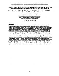
Figure 2. The histogram of training data samples (grey) and validating data samples (white) as a function of (a) Dst, (b) solar wind dynamic pressure, (c) interplanetary magnetic field (IMF) Bz, (d) IMF By, and (e) pitch angle. The last plot shows the histogram of difference between the neural network calculated L∗ and that obtained through the IRBEM library in the validating data set. Also shown are the standard deviation and mean difference between the two methods.

input conditions in the 27,000 samples. This distribution demonstrates a standard deviation as small as 0.06 and a mean difference near zero (∼ 10−5 ), indicating that the neural network is quite reliable in reproducing the L∗ value from IRBEM to reasonable accuracy. We evaluate the geomagnetic activity dependence of this L∗ neural network using the root-mean-square error (RMSE) as a function of solar wind dynamic pressure, Dst, and Bz (Table 1). The RMSE measures the difference between the artificial neural network (ANN) generated L∗ANN and IRBEM’s numerical tracing-based L∗IRBEM in response to the same input: √ √ N √1 ∑ RMSE = √ (L∗ − L∗IRBEM )2 (2) N i=1 ANN Except for extreme conditions such as Dst < −150 nT, Pdyn > 15 nPa, and |Bz| > 10 nT, the RMSE is mostly below 0.1, suggesting that for relatively quiet times or moderate storm periods, this neural network can reproduce L∗ with a fidelity comparable to the IRBEM-tracing method. However, caution may be needed when using the neural network for highly disturbed times because the neural network is trained from samples that have poor statistics under those highly disturbed conditions. Table 1. The Root-Mean-Square Error (RMSE) Between L∗ Calculated From the Neural Network Trained With the RAM-SCB Magnetic Field Configurations and L∗ Calculated From the IRBEM Library as a Function of Dst Index, Solar Wind Dynamic Pressure, and the Interplanetary Magnetic Field Bz Component Values

YU ET AL.

Dst (nT) samples RMSE

(> 0) 5488 0.055

(−50, 0) 20413 0.062

(−100, −50) 1357 0.101

(−150, −100) 70 0.147

Pdyn (nPa) samples RMSE

(0, 5) 26372 0.060

(5, 10) 944 0.088

(10, 15) 92 0.120

(15, 20) 22 0.178

(20, 25) 13 0.311

Bz (nT) samples RMSE

(>20) 9 0.164

(10, 20) 91 0.233

(0, 10) 13641 0.062

(−10, 0) 13571 0.062

(−20, −10) 91 0.107

©2014. American Geophysical Union. All Rights Reserved.

Overall

RMSE = 0.064

4

Journal of Geophysical Research: Space Physics

10.1002/2013JA019350

Figure 3. (top to bottom) L∗ computed from different artificial neural networks, L∗ computed from the IRBEM library, the relative difference between the above two methods, and the Dst index. The L∗ is calculated with different underlying magnetic field models including RAM-SCB, T89, T96, T01Storm, and T05. It is computed at a midnight location (−5.5, 0.0, 0.0) RE in SM coordinates with equatorial pitch angle of (left) 90◦ and (right) 50◦ .

We further compare this newly trained neural network with those previously trained from empirical magnetic field models, to discern any dependence of the L∗ outcome on the underlying magnetic field model. The neural network computed L∗ is also compared to that created by the IRBEM method. Figure 3 (left column) shows (a) L∗ANN , from five neural networks with different underlying magnetic field models, for a particle with 90◦ pitch angle starting at a midnight position (−5.5, 0, 0) RE during a small storm event. These neural networks provide similar L∗ values with disagreement mostly less than 0.7 between each other, implying that the neural network is not very sensitive to its underlying magnetic field model during small storm events and/or that the field models are not significantly different at these times. Also shown are (b) L∗ computed from the IRBEM method and (c) the relative difference between the two methods. The IRBEM-calculated L∗ values display similar results among different magnetic field models and the relative difference between the two methods is below 7%. While T96 model shows larger discrepancy in the storm main phase, the others have smaller differences (mostly below 3%) between the two methods. This again indicates the reliability of the neural network in reproducing IRBEM results in quiet or moderately disturbed time. Figure 3 (right column) shows the same parameters during the same event but for a pitch angle of 50◦ . Similarly, the L∗ difference either between different neural networks or between the two methods is small. However, this is not such a case in highly disturbed time (not shown) Because of the limitation of the neural network in representing extreme conditions, the uncertainty in the L∗ is significantly increased when Dst is below −150 nT. This suggests that for the above circumstances, the L∗ neural network is not as reliable as during less disturbed time. However, all of the underlying statistical magnetic field models themselves are least reliable during very active times. In this sense, a physics-based model could probably provide a better representation of the magnetospheric configuration for a specific storm event.

5. Estimating the Error of L∗ Calculation L∗ calculations are usually embedded with uncertainties, because such calculations are associated with a global magnetospheric field configuration produced by an empirical or physics-based magnetic field model, which itself has uncertainties that are difficult to quantify. An empirical global magnetic field model represents a statistical, average magnetosphere, while a physics-based first-principles model may include incomplete physical processes, and model uncertainty due to numerical approximation and discretization is

YU ET AL.

©2014. American Geophysical Union. All Rights Reserved.

5

Journal of Geophysical Research: Space Physics

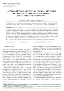
Figure 4. (top) The PSD observed by Van Allen Probes sorted in L∗ space during quiet time 3–4 January 2013 with 𝜇 = 2760 MeV∕G and K = 0.13 G1∕2 RE . (bottom) Black dots represent the matching ratio of two PSDs at conjunction points with the same adiabatic coordinates (𝜇 , K , L∗ ), and red triangles represent the L∗ error, |𝛿L∗ |, computed by equation (3). The neural network trained with T05 model is used for the L∗ calculation.

10.1002/2013JA019350

inevitable. The computed L∗ that carries the information of global magnetic fields thus accumulates these uncertainties, which is likely to influence the interpretation of the physics of the radiation belt [Green and Kivelson, 2004; Chen et al., 2007; Huang et al., 2008; McCollough et al., 2008; Yu et al., 2012]. Green and Kivelson [2004] discussed that L∗ uncertainties could result in a shift in the phase space density (PSD) radial profile, without changing its shape. This implies that the accuracy of L∗ could influence the determination of the PSD peak location or the location where the energization/acceleration of energetic electrons occurs in the inner magnetosphere.

Chen et al. [2007] developed a method for determining the accuracy of L∗ calculation by means of PSD-matching technique. Following equation (6) in Chen et al. [2007], the L∗ error can be quantified by ( )−1 𝜕f R−1 ∗ ̄ ∣ ∗ ∕2f ∣ ∣ 𝛿L ∣= R+1 𝜕L

(3)

Figure 5. Box-whisker plots of drift shell error 𝛿L∗ calculated from different neural networks at different 𝜇 values with K = 0.13 G1∕2 RE . The red line marks the median value of the error data set. The bottom and top of the box indicate 25th and 75th percentile, respectively. The whiskers extend to the most extreme data points within 1.5 times the interquartile range (IQR) outside the lower and upper quartiles. The numerical number under each box represents the median value ± MAD (median absolute deviation).

YU ET AL.

©2014. American Geophysical Union. All Rights Reserved.

6

Journal of Geophysical Research: Space Physics

10.1002/2013JA019350

Figure 6. (a) The distribution of L∗ , (b) the distribution of the phase space density (PSD), (c) local magnetic field magnitude at (−6.5, 0.0, 0.0) RE , and (d) PSD as a function of L∗ with 𝜇 = 523 MeV∕G and K = 0.11 G1∕2 RE , obtained from 100 magnetosphere configurations created by small random perturbations on the solar wind speed and density. The red dot represents the nominal value from the initial magnetosphere that experienced random disturbances. The T96 neural network is used for L∗ calculation.

where f represents the PSD value, R = f 2∕f 1 is the matching ratio between two PSD data under the same adiabatic coordinates, with the larger one always on the numerator, and f̄ = (f 1 + f 2)∕2 is the mean of the two PSD values. In order to use this technique, we should be aware of several sources causing the L∗ error. The reason for the two PSDs with the same adiabatic coordinates deviating from each other (i.e., the matching ratio R is not equal to one) can result from various error sources, including (1) inaccurate PSD conversion from flux observations especially in the fitting process (i.e., the fitting error source, as mentioned in Green and Kivelson [2004]), (2) inadequate satellite intercalibration, (3) large substorm injection that can violate the Liouville’s theorem based on which equation (3) is derived, (4) errors in the K parameter due to the imperfection of the magnetic field model, and (5) errors in the L∗ calculation due to the magnetic field model as well as the training process of the neural network. The error resulting from (1) can be much improved by using a cubic spline interpolation method in fitting an energy spectrum as reported in Yu et al. [2014]. To avoid, to a large extent, the potential contribution from error sources (2) and (3), only quiet time periods with small AL index are chosen for the L∗ error estimation, because the intersatellite “fine-tuned” calibration can produce trustworthy correction without large influence from substorm injection [Chen et al., 2005]. Finally, with the assumption that the uncertainty residing in the K parameter is much smaller than in L∗ , equation (3) is then used to evaluate the error of L∗ calculation originating from the neural network technique together with its corresponding underlying magnetic field model. Figure 4 demonstrates one example of the PSD at K ≃ 0.13 G1∕2 RE and 𝜇 ≃ 2760 MeV∕G calculated from electron flux measured by Energetic Particle, Composition, and Thermal Plasma (ECT)-Relativistic Electron-Proton Telescope (REPT) [Baker et al., 2013; Spence et al., 2013] onboard Van Allen Probes on 3–4 January 2013, the matching ratio R at conjunction points (i.e., same 𝜇 , K , L∗ ) between the two satellites and the computed drift shell error 𝛿L∗ . The REPT instruments are ideally suited to PSD-matching studies as they have been shown to be well cross calibrated [Morley et al., 2013]. This example employs the neural network with T05 magnetic field model to obtain the L∗ . The matching ratios R are mostly below 2.5 and 𝛿L∗ are mostly below 0.5. For a statistical estimate of 𝛿L∗ , we use a longer time period from 1 January through 28 February 2013 but exclude those days with AL index below −500 nT (substorm injections). The 𝛿L∗ is estimated using different neural networks and then is statistically analyzed in Figure 5 for three different 𝜇 YU ET AL.

©2014. American Geophysical Union. All Rights Reserved.

7

Journal of Geophysical Research: Space Physics

Figure 7. The PSD profile as a function of L∗ with K = 0.1 G1∕2 Re at different 𝜇 values. The five scattered clusters of data points (gray dots) correspond to PSD(L∗ ) distributions at five midnight equatorial positions (i.e., −6.0, −6.5, −7.0, −7.5, and −8.0 RE ). The blue dash line aligns the minimum L∗ from each data cluster, and the green dash line connects the maximum values. The red dot represents the nominal value from the initial magnetosphere that experienced random disturbances. The T96 neural network is used for L∗ calculation.

10.1002/2013JA019350

values. The box-whisker plot helps depict the degree of dispersion of the data: the bottom and the top of the box indicate the 25th and 75th percentile, respectively, with the range between the two being called the interquartile range (IQR). Figure 5 (middle red line) stands for the median value of the data, and the whiskers extend to the most extreme points within the range of 1.5 IQR outside the lower and upper quartile, respectively. The data above the top whisker are those on the tail of the distribution, larger than the 1.5 IQR plus the 75th percentile. When 𝜇 is larger the spread of the data set appears smaller (box is narrower), except in the RAM-SCB model, and the median value suggests a smaller 𝛿L∗ . Across different neural networks, 𝛿L∗ is similar. The median values are approximately around 0.2 with the median absolute deviation (MAD) within 0.11 and 0.17, and 75% (the top of the box) of the error distribution is mostly below 0.7. These results indicate that during relatively quiet time the L∗ computed from the neural network is reasonably accurate and little discrepancy exists between different neural networks. However, L∗ accuracy during highly disturbed time cannot be estimated using the above PSD-matching technique, because the Liouville’s theorem can be violated with sudden loss that usually occurs in storms.

6. L∗ Uncertainty Effect on PSD Profile As the error on the L∗ calculation from the neural network is approximately 0.2 ± 0.15 regardless of the underlying magnetic field model during relatively quiet times, the effect of such uncertainty on the radial profile of PSD is further investigated by using the neural network from the T96 field model for the L∗ calculation. We believe that the same conclusion can be drawn from using a different neural network, but here we only use one model to demonstrate the effect. While Green and Kivelson [2004] only qualitatively addressed the effect of L∗ uncertainty on the PSD radial profile, this work will quantitatively determine the influence on the PSD profile from a cluster of different L∗ values at different fixed positions. Given nominal solar wind conditions, a small perturbation is applied to both the solar wind velocity and density, resembling the uncertainty in solar wind measurements. This allows for the generation of a different magnetosphere configuration, resulting in a range of calculated L∗ . The artificial fluctuation in the solar wind condition mimics the measurement uncertainty of solar wind speed and density, which are approximately 1% and 15%, respectively (R. Skoug and J. Steinberg, personal communication, 2013; see also http://omniweb.gsfc.nasa. gov/html/omni2_doc.html by Joe King and Natalia Papitashvili). An ensemble of 100 small disturbances is applied to both the nominal solar wind density and speed, generating a pseudo-normal distribution around the nominal condition with the above uncertainty (1%, 15%) as their standard deviation, respectively. Based on these magnetospheric configurations, L∗ is calculated from the neural network at several different locations ranging from 6.0 to 8.0 RE on the midnight Sun-Earth line. The corresponding PSD at these positions YU ET AL.

©2014. American Geophysical Union. All Rights Reserved.

8

Journal of Geophysical Research: Space Physics

10.1002/2013JA019350

is converted from nominal energy differential electron flux, which is obtained from the AE-8 radiation belt model with different energy and pitch angle for solar minimum conditions, following the conversion procedure described in Yu et al. [2014]. As an example, at location of (−6.5, 0, 0) RE L∗ and PSD both display a pseudo-normal distribution (Figures 6a and 6b); the local magnetic field and PSD generally increase monotonically with L∗ (Figures 6c and 6d). A change of 3% in the magnetic field results in a change of 3% in L∗ value and a change of 12% in the PSD at this selected location. It should be noted that the degree of change in the PSD depends on the PSD radial gradient at the position of interest. Figure 7 collects the PSD(L∗ ) results computed at different locations on the midnight equator based on the above 100 magnetospheric configurations. At each location, a scatter of PSD(L∗ ) distributes around the nominal result (Figure 7, red dot), representing the associated uncertainty. The uncertainties in the PSD and L∗ therefore envelope a radial span in the PSD profile, with the blue line aligning the minimum L∗ values and the green one aligning the maximum values from each scattered cluster. Between these two extrema, the shape of the PSD profile seems to persist, but the peak location is shifted approximately by 0.2 in L∗ . This finding is quantitatively consistent with the conclusion in Green and Kivelson [2004]. The PSD radial profile at different 𝜇 values suggests that the PSD radial gradient is energy dependent. This feature is also preserved even with the uncertainty in L∗ . While the above ensemble of magnetosphere configurations can mostly be considered as quiet systems and the variability in both the L∗ and PSD is not significant, a storm-time magnetosphere would result in a larger uncertainty in L∗ and hence a stronger shift in the PSD radial profile would be expected. Nevertheless, the above experiment may shed some light on the potential impact on the interpretation of the underlying physics in the radiation belt, such as the responsible energization mechanism for creating the localized PSD peak.

7. Summary As a continuing effort on increasing the computational capability of efficiently, accurately obtaining L∗ , this study trains the L∗ neural network based on the first-principles magnetic field configuration from RAM-SCB model, with simple inputs including solar wind conditions and the Dst index, which allows for a much easier preparation of inputs than the previous L∗ networks that require the McIlwain L and the magnetic field at the mirror point as part of the inputs. The newly trained neural network is compared against the previously trained neural networks from empirical magnetic field models as well as the tracing method in the IRBEM library and is found to reasonably agree with other L∗ values during moderate storm events and quiet times. But the difference in the L∗ is substantially increased across all these neural networks during large storms. This is probably attributed to insufficient statistics for the extreme cases to result in a reliabler neural network. The accuracy of L∗ neural networks with different underlying magnetic field models (both empirical and physics based) is estimated with the PSD-matching technique using Van Allen Probes observations. The median value of the drift shell error is approximately around 0.2 with median absolute deviation (MAD) around 0.15 during relatively quiet time for all the neural networks. The uncertainty in the calculated L∗ value is found to affect the PSD profile by shifting it radially without changing its shape, which implies its influence on the interpretation of radiation belt physics such as localized energization.

Acknowledgments We gratefully acknowledge the support of the U.S. Department of Energy through the Los Alamos National Laboratory (LANL)/Laboratory Directed Research and Development (LDRD) program, as well as the support of NASA through NNH10APOGI and NNG13PJ05I and NSF through IA1203460. Masaki Fujimoto thanks the reviewers for their assistance in evaluating this paper.

YU ET AL.

References Baker, D., et al. (2013), The relativistic electron-proton telescope (REPT) instrument on board the radiation belt storm probes (RBSP) spacecraft: Characterization of Earth’s radiation belt high-energy particle populations, Space Sci. Rev., 179, 337–381, doi:10.1007/s11214-012-9950-9. Chen, Y., R. H. W. Friedel, G. D. Reeves, T. G. Onsager, and M. F. Thomsen (2005), Multisatellite determination of the relativistic electron phase space density at geosynchronous orbit: Methodology and results during geomagnetically quiet times, J. Geophys. Res., 110, A10210, doi:10.1029/2004JA010895. Chen, Y., R. H. W. Friedel, G. D. Reeves, T. E. Cayton, and R. Christensen (2007), Multisatellite determination of the relativistic electron phase space density at geosynchronous orbit: An integrated investigation during geomagnetic storm times, J. Geophys. Res., 112, A11214, doi:10.1029/2007JA012314. Gannon, J. L., S. R. Elkington, and T. G. Onsager (2012), Uncovering the nonadiabatic response of geosynchronous electrons to geomagnetic disturbance, J. Geophys. Res., 117, A10215, doi:10.1029/2012JA017543. Green, J. C., and M. G. Kivelson (2004), Relativistic electrons in the outer radiation belt: Differentiating between acceleration mechanisms, J. Geophys. Res., 109, A03213, doi:10.1029/2003JA010153. Henderson, M. G., S. K. Morley, and B. A. Larsen (2011), LANLGeoMag, version 1.5.13, Tech. Rep. LA-CC-11-104, Los Alamos National Laboratory, Los Alamos, N. M.

©2014. American Geophysical Union. All Rights Reserved.

9

Journal of Geophysical Research: Space Physics

10.1002/2013JA019350

Huang, C.-L., H. E. Spence, H. J. Singer, and N. A. Tsyganenko (2008), A quantitative assessment of empirical magnetic field models at geosynchronous orbit during magnetic storms, J. Geophys. Res., 113, A04208, doi:10.1029/2007JA012623. Jordanova, V. K., J. U. Kozyra, G. V. Khazanov, A. F. Nagy, C. E. Rasmussen, and M.-C. Fok (1994), A bounce-averaged kinetic model of the ring current ion population, Geophys. Res. Lett., 21, 2785–2788, doi:10.1029/94GL02695. Jordanova, V. K., Y. S. Miyoshi, S. Zaharia, M. F. Thomsen, G. D. Reeves, D. S. Evans, C. G. Mouikis, and J. F. Fennell (2006), Kinetic simulations of ring current evolution during the Geospace Environment Modeling challenge events, J. Geophys. Res., 111, A11S10, doi:10.1029/2006JA011644. Jordanova, V. K., S. Zaharia, and D. T. Welling (2010), Comparative study of ring current development using empirical, dipolar, and self-consistent magnetic field simulations, J. Geophys. Res., 115, A00J11, doi:10.1029/2010JA015671. Koller, J., and S. Zaharia (2011), LANL* V2.0: Global modeling and validation, Geosci. Model Dev., 4(1), 669–675, doi:10.5194/gmd-4-669-2011. Koller, J., Y. Chen, G. D. Reeves, R. H. W. Friedel, T. E. Cayton, and J. A. Vrugt (2007), Identifying the radiation belt source region by data assimilation, J. Geophys. Res., 112, A06244, doi:10.1029/2006JA012196. Koller, J., G. D. Reeves, and R. H. W. Friedel (2009), LANL* V1.0: A radiation belt drift shell model suitable for real-time and reanalysis applications, Geosci. Model Dev., 2, 113–122. McCollough, J. P., J. L. Gannon, D. N. Baker, and M. Gehmeyr (2008), A statistical comparison of commonly used external magnetic field models, Space Weather, 6, S10001, doi:10.1029/2008SW000391. Min, K., J. Bortnik, and J. Lee (2013a), A novel technique for rapid L∗ calculation using UBK coordinates, J. Geophys. Res. Space Physics, 118, 192–197, doi:10.1029/2012JA018177. Min, K., J. Bortnik, and J. Lee (2013b), A novel technique for rapid L∗ calculation: Algorithm and implementation, J. Geophys. Res. Space Physics, 118, 1912–1921, doi:10.1002/jgra.50250. Morley, S. K., M. G. Henderson, G. D. Reeves, R. H. W. Friedel, and D. N. Baker (2013), Phase space density matching of relativistic electrons using the Van Allen Probes: REPT results, Geophys. Res. Lett., 40, 4798–4802, doi:10.1002/grl.50909. Reeves, G. D., et al. (2013), Electron acceleration in the heart of the Van Allen radiation belts, Science, 341, 991–994, doi:10.1126/science.1237743. Roederer, J. G. (1970), Dynamics of Geomagnetically Trapped Radiation, Physics and Chemistry in Space, Springer, Berlin. Selesnick, R. S., and J. B. Blake (1998), Radiation belt electron observations following the January 1997 magnetic cloud event, Geophys. Res. Lett., 25(14), 2553–2556, doi:10.1029/98GL00665. Spence, H., et al. (2013), Science goals and overview of the radiation belt storm probes (RBSP) energetic particle, composition, and thermal plasma (ECT) suite on NASA’s Van Allen Probes mission, Space Sci. Rev., 179(1–4), 311–336, doi:10.1007/s11214-013-0007-5. Stern, D. P. (1975), The motion of a proton in the equatorial magnetosphere, J. Geophys. Res., 80, 595–599, doi:10.1029/JA080i004p00595. Tsyganenko, N. A. (1989), A magnetospheric magnetic field model with a warped tail current sheet, Planet. Space Sci., 37, 5–20, doi:10.1016/0032-0633(89)90066-4. Tsyganenko, N. A., and M. I. Sitnov (2005), Modeling the dynamics of the inner magnetosphere during strong geomagnetic storms, J. Geophys. Res., 110, A03208, doi:10.1029/2004JA010798. Turner, D. L., Y. Shprits, M. Hartinger, and V. Angelopoulos (2012), Explaining sudden losses of outer radiation belt electrons during geomagnetic storms, Nat. Phys., 8, 208–212, doi:10.1038/nphys2185. Volland, H. (1973), A semiempirical model of large-scale magnetospheric electric fields, J. Geophys. Res., 78, 171–180, doi:10.1029/JA078i001p00171. Weimer, D. R. (2001), An improved model of ionospheric electric potentials including substorm perturbations and application to the Geospace Environment Modeling November 24, 1996, event, J. Geophys. Res., 106, 407–416, doi:10.1029/2000JA000604. Yu, Y., J. Koller, S. Zaharia, and V. Jordanova (2012), L∗ neural networks from different magnetic field models and their applicability, Space Weather, 10, S02014, doi:10.1029/2011SW000743. Yu, Y., J. Koller, V. Jordanova, S. Zaharia, and H. Godinez (2014), Radiation belt data assimilation of a moderate storm event using the physics-based magnetic field configuration from RAM-SCB, Ann. Geophys., doi:10.5194/angeo-2013-264-2014, in press. Zaharia, S. (2008), Improved Euler potential method for three-dimensional magnetospheric equilibrium, J. Geophys. Res., 113, A08221, doi:10.1029/2008JA013325. Zaharia, S., C. Cheng, and K. Maezawa (2004), 3-D force-balanced magnetospheric configurations, Ann. Geophys., 22, 251–265, doi:10.5194/angeo-22-251-2004. Zaharia, S., V. K. Jordanova, M. F. Thomsen, and G. D. Reeves (2006), Self-consistent modeling of magnetic fields and plasmas in the inner magnetosphere: Application to a geomagnetic storm, J. Geophys. Res., 111, A11S14, doi:10.1029/2006JA011619.

YU ET AL.

©2014. American Geophysical Union. All Rights Reserved.

10