Research
A Section 508–conformant HTML version of this article is available at http://dx.doi.org/10.1289/EHP190.
Assessing Temporal and Spatial Patterns of Observed and Predicted Ozone in Multiple Urban Areas Heather Simon, Benjamin Wells, Kirk R. Baker, and Bryan Hubbell Office of Air Quality Planning and Standards, U.S. Environmental Protection Agency, Research Triangle Park, North Carolina, USA
Background: Ambient monitoring data show spatial gradients in ozone (O3) across urban areas. Nitrogen oxide (NOx) emissions reductions will likely alter these gradients. Epidemiological studies often use exposure surrogates that may not fully account for the impacts of spatially and temporally changing concentrations on population exposure. Objectives: We examined the impact of large NOx decreases on spatial and temporal O3 patterns and the implications on exposure. Methods: We used a photochemical model to estimate O3 response to large NOx reductions. We derived time series of 2006–2008 O3 concentrations consistent with 50% and 75% NOx emissions reduction scenarios in three urban areas (Atlanta, Philadelphia, and Chicago) at each monitor location and spatially interpolated O3 to census-tract centroids. Results: We predicted that low O3 concentrations would increase and high O3 concentrations would decrease in response to NOx reductions within an urban area. O3 increases occurred across larger areas for the seasonal mean metric than for the regulatory metric (annual 4th highest daily 8-hr maximum) and were located only in urban core areas. O3 always decreased outside the urban core (e.g., at locations of maximum local ozone concentration) for both metrics and decreased within the urban core in some instances. NOx reductions led to more uniform spatial gradients and diurnal and seasonal patterns and caused seasonal peaks in midrange O3 concentrations to shift from midsummer to earlier in the year. Conclusions: These changes have implications for how O3 exposure may change in response to NOx reductions and are informative for the design of future epidemiology studies and risk assessments. Citation: Simon H, Wells B, Baker KR, Hubbell B. 2016. Assessing temporal and spatial patterns of observed and predicted ozone in multiple urban areas. Environ Health Perspect 124:1443–1452; http://dx.doi.org/10.1289/EHP190
Introduction Exposure to ozone (O3) is known to cause negative health effects in humans [U.S. Environmental Protection Agency (EPA) 2013]. Many areas in the United States currently experience O3 concentrations that exceed the National Ambient Air Quality Standards (NAAQS) (https://ozoneair qualitystandards.epa.gov/OAR_OAQPS/ OzoneSliderApp/index.html#). Although there have been substantial emission reductions of O3 precursors, and peak O3 concentrations have decreased as a result of these reductions, some areas are expected to continue to exceed the 8-hr O3 NAAQS in the future (U.S. EPA 2014b). Nitrogen oxide (NO x ) and volatile organic compound (VOC) emissions react in the atmosphere through complex nonlinear chemical reactions to form ground-level O3 when meteorological conditions are favorable (Seinfeld and Pandis 2012). Specifically, NOx participates in chemical pathways for both O3 formation and destruction; therefore, the net impact of NOx emissions on O3 concentrations depends on the relative abundances of NO x, VOCs, and sunlight as well as on the temporal and spatial scales being examined. Emissions sources of NOx and VOC and the resulting O3 vary seasonally, diurnally, and spatially. Spatial differences exist from rural to urban, city to city,
and even within a given urban area (Marshall et al. 2008). In locations with high concentrations of nitric oxide (NO), one component of NO x, O 3 can become artificially suppressed owing to direct reactions of NO with O3. These reactions also result in the production of other oxidized nitrogen species, which form O 3 away from the emission source location while the wind transports the air mass, thus contributing to elevated O3 downwind (Cleveland and Graedel 1979). As a result of this chemistry, decreasing NOx and VOC emissions generally decrease O3 at times and locations in which O3 concentrations are high (Simon et al. 2013). In limited circumstances, reductions of NOx emissions can lead to O3 increases in the immediate vicinity of highly concentrated NOx sources, whereas these same emissions changes generally lead to reductions of O3 downwind over longer timescales (Cleveland and Graedel 1979; Kelly et al. 2015; Murphy et al. 2007; Sillman 1999; Xiao et al. 2010). Because emissions of both NOx and VOC decrease from sources that have unique temporal and spatial attributes (e.g., power plant NOx and mobile source NOx and VOCs), it will be important to characterize how O3 formation regimes vary over different temporal and spatial scales in order to understand how O3 concentrations may change as a result of these emissions reductions.
Environmental Health Perspectives • volume 124 | number 9 | September 2016
Spatial and temporal variability in pollutant concentrations are key inputs to studies evaluating associations between air quality and human health. In the past, epidemiological studies linking O 3 with human health impacts have used ambient measurements in various ways to match against health outcomes. Some studies have used spatially averaged O3 concentrations for an entire urban area to link with short-term (Smith et al. 2009; Zanobetti and Schwartz 2008) and long-term (Jerrett et al. 2009) mortality. Other studies have used the O3 monitor closest to the residence of the human subjects (Bell 2006). The use of an average “composite” monitor masks both spatial and temporal heterogeneity that exist in an urban area. Using the nearest monitor may provide a better spatial match but does not fully consider daily activity patterns. Given the spatial and temporal heterogeneity in O3 and human activity patterns that place a subject in different places at different times of the day, it is potentially important to match activity with a realistic heterogeneous representation of O3 concentrations. This is true for conducting epidemiology studies of O3 health outcomes, as well as in the application of the results of those studies in risk and health impact assessments. To the extent that reductions in NOx and VOC emissions change the temporal and spatial patterns of O3, the use of a spatially averaged O3 concentration may mask how population-weighted O3 exposures change. Recent risk assessments conducted to inform the U.S. EPA review of the O3 NAAQS included application of results from both controlled human exposure studies and observational epidemiology studies (U.S. EPA 2014a). Estimates of risk based on controlled human exposure studies evaluated changes Address correspondence to H. Simon, 109 T.W. Alexander Dr., Research Triangle Park, NC 27711 USA. Telephone: (919) 541-1803. E-mail: simon.
[email protected] Supplemental Material is available online (http:// dx.doi.org/10.1289/EHP190). The authors would like to thank N. Possiel, A. Lamson, K. Scavo, J. Hemby, K. Bremer, and M. Koerber at the U.S. Environmental Protection Agency (EPA) for their thoughtful review and comments on this article. Although this paper has been reviewed by the U.S. EPA and approved for publication, it does not necessarily reflect the U.S. EPA’s policies or views. The authors declare they have no actual or potential competing financial interests. Received: 16 October 2015; Revised: 17 December 2015; Accepted: 27 April 2016; Published: 6 May 2016.
1443
Simon et al.
in the risk of 10% and 15% lung function decrements and used an exposure–response model that was more responsive to changes in exposure when the maximum daily 8-hr average (MDA8) O 3 was > 40 ppb. In contrast, estimates of risk based on the application of results from epidemiology studies used linear, no-threshold concentration– response functions, so an incremental change in O3 affected total risk equally, regardless of the starting level of O3. As a result, the epidemiology-based risk estimates could be quite sensitive to the patterns of O3 responses to NOx reductions, whereas the risk estimates based on controlled human exposure studies reflected the changes that occurred at the higher O3 concentrations. Given the complex nature of O3 chemistry and emissions source mixes in a given urban area, photochemical grid models provide a credible tool for evaluating responsiveness to emissions changes and have been used extensively for O3 planning purposes in the past
(Cai et al. 2011; Hogrefe et al. 2011; Kumar and Russell 1996; Simon et al. 2012). In the present study, we used a photochemical grid model applied in three different urban areas to illustrate temporal and spatial patterns of O3 and how those patterns may change as a result of reduced precursor emissions. Modelpredicted changes in O3 were aggregated using several metrics to show how spatial heterogeneity depends on the O3 metric that is being analyzed and how the type of aggregation used can mute the spatial variability in O3 response to emissions changes.
Methods City Selection And Monitoring Data Three major urban areas (Philadelphia, Atlanta, and Chicago) were selected for evaluation based on the spatial coverage of the local ambient monitoring network and because they demonstrate different types of spatial O3 patterns and responses to emissions
changes (U.S. EPA 2014a). In addition, the photochemical model performed well in these cities (U.S. EPA 2014a). For each urban area, all ambient monitoring sites within the combined statistical area (CSA) were included in the analysis as well as any additional monitoring sites within a 50-km buffer of the CSA boundary. Hourly average O 3 data from these ambient monitoring sites for the years 2006–2008 were obtained from the U.S. EPA’s Air Quality System (AQS) database (http://www2.epa.gov/aqs).
Ambient Data Adjustments to Estimate O3 Distributions under Alternate Emissions We applied outputs from a series of photochemical air quality model simulations to estimate how hourly O3 could change under hypothetical scenarios of 50% and 75% reductions in U.S. anthropogenic NOx emissions. Emissions projections from the U.S. EPA predict substantial reductions (45%)
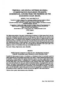
Figure 1. Maps showing the 2006–2008 average annual 4th-highest maximum daily 8-hr average ozone (MDA8 O3), the regulatory metric (parts per billion; top panels), and May–September mean MDA8 O3 (parts per billion; bottom panels) values in Atlanta for observed conditions (left panels), and predicted changes with 50% U.S. nitrogen oxide (NOx) emissions reductions (center panels) and 75% U.S. NOx emissions reductions (right panels). Colored squares show locations of monitoring sites, and colored dots show interpolated values at census-tract centroids.
1444
volume
124 | number 9 | September 2016 • Environmental Health Perspectives
Temporal and spatial O3 patterns in three urban areas
in U.S. anthropogenic NOx between 2007 and 2020 (U.S. EPA 2012). VOC emissions are also expected to decline between 2007 and 2020 by a more modest 20% (U.S. EPA 2012). By evaluating O3 concentrations at 50% and 75% NOx reductions, we were able to look at O3 responses for two scenarios of varying emissions. Although the primary focus of this study was on NOx reduction scenarios, we also included a more limited evaluation of scenarios where both NOx and VOC emissions were reduced by 50% and 75% to determine how cooccurring VOC reductions could change patterns of responses to NOx reductions. The methodology for adjusting observed O3 to scenarios of 50% and 75% NOx reductions was adapted from the methods developed by Simon et al. (2013) and by the U.S. EPA (2014a). However, both of these studies targeted specific air quality goals rather than emissions reduction levels as were investigated
here. The methods are described in detail in those documents and are summarized below. We used the Community Multi-scale Air Quality (CMAQ) model v.4.7.1 instrumented with higher-order decoupled direct method (HDDM) capabilities to calculate O3 responses to emissions inputs. Details on the model setup and inputs are provided in the Supplemental Material (“Supplemental Methods”). Model predictions of MDA8 O3 were compared with monitored values in each of the three cities. Overall, the mean biases were 3.7 ppb, 2 ppb, and 1 ppb in Atlanta, Chicago, and Philadelphia, respectively. The Pearson correlations (R) were 0.82, 0.86, and 0.88, respectively. A seasonal breakout of these performance statistics is provided in Table S1. This model performance is within the range of what has been observed in state-of-the-science ozone modeling reported in recent studies (Simon et al. 2012) and is sufficiently accurate for the purpose of this analysis.
The CMAQ-HDDM system provided outputs of hourly O3 and hourly sensitivity coefficients at a 12 km × 12 km grid resolution across the contiguous United States. These sensitivities describe a nonlinear (quadratic) O3 response at a specified time and location to an across-the-board perturbation in NOx emissions following Equation 1:
1 DO3 h,l = - DfS h,l +
Df 2 2 2 S h,l , [1]
where ∆O3 h,l is the change in O3 at hour h and location l, ∆ε is the relative change in NOx emissions (e.g., –0.2 represents a 20% reduction in NO x emissions) and S 1h,l and 2 S h,l represent the first- and second-order O3 sensitivity coefficients at hour h and location l. Model simulations were performed for 7 months in 2007 (January and April– October), which provided O 3 responses over a range of emissions and meteorological conditions and provided information on
Figure 2. Maps showing the 2006–2008 average annual 4th-highest maximum daily 8-hr average ozone (MDA8 O 3), the regulatory metric, (parts per billion; top panels) and May–September mean MDA8 O3 (parts per billion; bottom panels) values in Philadelphia for observed conditions (left panels), and predicted changes with 50% U.S. nitrogen oxide (NOx) emissions reductions (center panels) and 75% U.S. NOx emissions reductions (right panels). Colored squares show locations of monitoring sites, and colored dots show interpolated values at census-tract centroids.
Environmental Health Perspectives • volume 124 | number 9 | September 2016
1445
Simon et al.
seasonal variations in the response. To apply the modeled sensitivity coefficients from 7 months to 3 years of ambient measurements (described above), we derived statistical relationships between the modeled sensitivity coefficients and the modeled hourly O3 concentrations using linear regression. Separate linear regressions were created for each monitor location at each hour of the day and for each season, resulting in a total of 96 (24 hr × 4 seasons) linear regressions for the first- and second-order sensitivity coefficients at each monitor location. The linear regression resulted in statistically significant relationships between ozone concentration and responsiveness to NOx emissions reductions for most combinations of hours of the day, season, and monitoring location. Using these relationships, we could determine the first- and second-order sensitivity coefficients at O3 monitor locations for every hour of 2006–2008. Finally, we used Equation 1
to predict the change in measured ambient O3 concentrations for a set change in NOx emissions at each monitor location. An additional complication is introduced when looking at large changes in NOx emissions (e.g., 50% and 75%). Previous studies have reported that CMAQ-HDDM estimates of O3 changes are most accurate for emissions perturbations