AbstractâWe present a method to automatically detect shadows in a fast and accurate ... We can thus build an accurate shadow candidate map based on.
IEEE TRANSACTIONS ON PATTERN ANALYSIS AND MACHINE INTELLIGENCE, VOL. , NO. ,
1
Automatic and accurate shadow detection using near-infrared information ´ Dominic Rufenacht, Student Member, IEEE, Clement Fredembach, and Sabine Susstrunk, Senior ¨ ¨ Member, IEEE Abstract—We present a method to automatically detect shadows in a fast and accurate manner by taking advantage of the inherent sensitivity of digital camera sensors to the near-infrared (NIR) part of the spectrum. Dark objects, which confound many shadow detection algorithms, often have much higher reflectance in the NIR. We can thus build an accurate shadow candidate map based on image pixels that are dark both in the visible and NIR representations. We further refine the shadow map by incorporating ratios of the visible to the NIR image, based on the observation that commonly encountered light sources have very distinct spectra in the NIR band. The results are validated on a new database, which contains visible/NIR images for a large variety of real-world shadow creating illuminant conditions, as well as manually labelled shadow ground truth. Both quantitative and qualitative evaluations show that our method outperforms current state-of-the-art shadow detection algorithms in terms of accuracy and computational efficiency. Index Terms—Shadow detection, near-infrared.
F
1
I NTRODUCTION
A
Shadow is created when an object lies in the path of a light source. Shadows are cast by the occluding object, or the object itself can be shaded; a phenomenon known as “self-shading”. Due to the difference between the light intensity reaching a shaded region and a directly lit region, shadows are often characterized by strong brightness gradients. While non-shadow regions are illuminated by both direct (e.g., sunlight, flashlight) and diffuse (e.g., skylight, fluorescent, incandescent) light sources, shadow regions are only illuminated by diffuse light. The change between shadow and non-shadow regions is thus not only a brightness difference, but a color one as well. In outdoor scenes, for example, the lit areas are illuminated by sunlight and skylight, while the shadow regions are illuminated by skylight alone, which creates a bluish color cast. This property of shadows, together with the fact that a certain color can exist in both lit and shaded objects, makes them problematic in a number of different computer vision applications such as tracking [1], object (or people) recognition [2], and white-balancing [3]. In image manipulation or compositing, shadows are often unwanted artefacts that are unavoidable due to image capture conditions (e.g., photographs taken in an urban environment). While shadow compositing and removal has dramatically improved in recent years [4], [5], [6], [7], automatic shadow detection is still a challenge and requires additional assumptions or information. Our proposed approach starts with the fact that camera • D. Rufenacht, ¨ C. Fredembach, and S. Susstrunk ¨ are with the School of Computer and Communication Sciences, Ecole Polytechnique F´ed´erale de Lausanne (EPFL), Lausanne, Switzerland. E-mail: {dominic.ruefenacht,clement.fredembach,sabine.susstrunk}@epfl.ch.
sensors are inherently sensitive to the near-infrared (NIR) spectrum (700–1100 nm). The algorithm is based on three observations: First, shadows are generally darker than their surroundings, in both the visible and the NIR. Second, the majority of objects that are dark in the visible spectrum are much brighter in NIR. Third, most of the considered illuminants in the shadow formation process have a distinct behavior in the NIR. These observations lead to a shadow detection framework that takes visible and NIR images as input and produces accurate binary shadow masks. Comparing our results with two state-of-the-art shadow detection methods [8], [9], we show that our algorithm performs better on average, is more robust (less performance variation image-wise), and is faster. The algorithm works best with unprocessed (linear) RAW images. The method, however, also provides very good results on images already processed in-camera. Thus, the only requirement is that both visible and NIR information is available. Combining visible and NIR images has been successfully used to improve various image processing and computer vision tasks, such as skin smoothing [10], high dynamic range image rendering [11], haze removal [12], [13], scene recognition [14], and semantic region labeling [15]. In addition, enabling simultaneous capture of both visible and NIR radiation with a single sensor [16], [17] is currently being researched. Because our method is computationally inexpensive and works on RAW images, it can easily be implemented in-camera to provide assistance where shadow detection is beneficial, e.g., white-balancing or automatic image enhancement.
IEEE TRANSACTIONS ON PATTERN ANALYSIS AND MACHINE INTELLIGENCE, VOL. , NO. ,
2
R ELATED W ORK
Image-based shadow detection algorithms can loosely be classified into two categories based on the type of additional information they employ: Semi-automatic methods that require some type of user input, and fully automatic methods, which often make additional, constraining assumptions about the scene in order to work properly. 2.1
Semi-Automatic Methods
A common way to sidestep the difficulty of automatic shadow detection is to assist the detection algorithm with user-supplied information. A number of recent and well-performing methods incorporate user input to either “seed” or correct the detection process. In Wu et al. [6], users are asked to submit a quad-map containing shadow, non-shadow, and penumbra regions of similar textures. Simplifications of these user requirements are focused towards reducing the time spent selecting shadow and non-shadow regions. Wu and Tang [18] employ user-supplied context that indicates candidate shadow regions. Arbel and Hel-Or’s method [4] allows a shadow mask to be calculated using only a few keypoints, and Shor and Lischinski [5] proposed reducing external information to one user-supplied keypoint per shadow region. Instead of “growing” a shadow region based on a few keypoints, Drew and Reza [19] calculate invariant images based on a few selected patches in the image. While these detection algorithms can provide very accurate results for still images and deliver good subsequent shadow removal, their requirements are strongly dependent on the complexity of the image. Moreover, even minimal user interaction prevents a detection algorithm to be incorporated in a fully automatic workflow, such as in-camera image processing. 2.2
Fully Automatic Methods
2.2.1 Single-Image Approaches Automatic shadow detection on single images has been addressed in a variety of approaches. Gradient-based methods, where edges are classified as either shadow or material transitions depending on their direction and magnitudes, have been proposed in [20], [21]. Assuming Planckian illumination, Finlayson et al. [22], [23] showed that greyscale illumination-invariant images could be obtained by projecting an image’s log chromaticities in an appropriate direction, found by either calibration [22] or entropy minimization [23]. Comparing the edge content of the original image with the edges of the invariant one effectively yields shadow edges. Despite their relatively simple assumptions, these methods often work well and still are among state-of-the-art regarding automatic shadow detection from a single image. However, they do not account for simultaneous material/illumination changes, which can limit their usefulness in more complex scenes. Lalonde et al. [7] propose an algorithm that automatically detects ground shadows
2
in consumer-grade photographs. Limiting the algorithm to cast shadows on the ground allows them to focus on a limited set of materials and learn the shadow appearance on those materials from a labelled set of images. Tian et al. [24] make similar assumptions to [22], but in addition employ a trichromatic attenuation model (TAM). They first oversegment the image, and then apply the TAM model to decide whether a segment is in the shadow or not. The use of several thresholds, however, makes this approach fairly unstable. In [8], they improve the TAM model, no longer use segmentation and only compute a single threshold, which yields much improved results. Different to the previous methods, Guo et al. [9] explicitly model the material and illumination relationships of pairs of regions. They employ a segmentation-based approach, and learn their classifiers from training data. Both [8] and [9] compute a binary shadow mask, which allows for a fair comparison to our method.
2.2.2
Multi-Image Approaches
To minimize the ambiguities induced by simultaneous material and illumination changes, some research has focused on multi-image methods. For instance, flash/noflash image pairs can be combined to either estimate the illuminant [25], [26], or to remove shadows [27]. The chromagenic illuminant estimation of Finlayson et al. [28] postulates that capturing two images of a given scene, using a broadband colored filter to capture the second image, and comparing them adequately, produces accurate illumination maps. In the right context, these multiimage algorithms perform remarkably well, although their context can be limited: flash cannot illuminate all outdoor shadows, and the chromagenic approach requires image segmentation, an accurate training step, and every pair of trained illuminants needs to be tested. On the other hand, the chromagenic approach is not limited to shadows, and can incorporate a number of multi-illuminant scenes. Closer to our method, Teke et al. [29] create a falsecolor image of satellite imagery by replacing the blue channel of the RGB image with NIR. By analyzing the difference between saturation and intensity of the falsecolor image, and subsequent independent processing of vegetation regions, they are able to obtain shadow maps for remote sensing applications. While their method employs near infrared information, it does not make use of its relationship to the visible spectrum and is limited to remote sensing environments. Currently, we use a multi-image approach, as we capture the visible and the NIR part of the spectrum separately. The feasibility of a visible plus NIR sensor shown in [16], [17] motivates our belief that in the near-future, digital camera sensors will jointly capture visible and NIR, which will turn our method into a single-image approach.
IEEE TRANSACTIONS ON PATTERN ANALYSIS AND MACHINE INTELLIGENCE, VOL. , NO. ,
3
Fig. 1: Our proposed framework. We use both information from the visible and the NIR part of the spectrum to compute a shadow candidate map. The results are refined by combining this map with a color to NIR ratio map. The shadow map is thresholded to obtain a binary shadow mask.
3
N EAR - INFRARED I MAGING
Silicon, the photosensitive component of a digital camera’s sensor, is intrinsically sensitive not only to visible light (∼400–700 nm), but also to NIR (∼700–1100 nm). In fact, its sensitivity is such that a specifically designed filter (often called a hot mirror) has to be placed in front of the sensor to prevent NIR contamination of the visible images. This filter is necessary for both monochromatic and color cameras, because the filter colorants employed to create the color filter array (CFA) are also transparent to the NIR. Fig. 2a shows the normalized quantum efficiencies we measured of a Canon EOS 5D Mark II without its hot mirror. By removing the hot mirror, both
EOS 5D Mark II with a sequential approach to capture the visible/NIR image pairs. Figures 2b and 2c show the measured quantum efficiency of the camera with filters placed in front of the lens. Samples of color/NIR image pairs can be found in Fig. 7.
4
S HADOW D ETECTION A LGORITHM
Shadows are, almost by definition, darker than their surroundings. However, just equating shadows with dark regions is shortsighted because all dark objects will become potential shadows and result in imprecise shadow masks. NIR possesses some important properties that make the shadow candidate selection more accurate. Spectral studies of natural and man-made surfaces and colorants [30], [31], [32] show that in general: Z Z R,G,B S(λ)Q (λ)dλ < S(λ)QN IR (λ)dλ, (1) V IS
(a)
(b)
(c)
Fig. 2: Measured quantum efficiencies of red, green, and blue of a Canon EOS 5D Mark II without hot mirror and (a) no filter, (b) with a NIR-blocking filter (B+W 486), and (c) with a visible light blocking filter (B+W 093). The quantum efficiencies are normalized to 1.
the visible and NIR part of the spectrum can be captured. However, in order to obtain useful information, the visible and NIR signals that reach the imaging sensor need to be separated. One way of doing so is to employ a beamsplitter to separate visible wavelengths from NIR ones and two (or more) cameras or sensors to capture a portion of the spectrum only [11]. This method is quite expensive, and has a substantial light loss induced by the beamsplitter. Another, single camera approach consists in first capturing a color image by putting a NIR-blocking filter in front of the lens, and then an NIR image by placing a visible light blocking filter in front of the lens. In this work, we used a characterized Canon
N IR
i.e., the reflectance S(λ) times quantum efficiency Q(λ) in the NIR is greater than in any of the RGB channels. Two notable exceptions are water, which has an absorption band in the NIR, and carbon black, a colorant often encountered in black plastic objects, where both NIR and the visible bands have a similar, almost zero reflectance. The implication of Equation 1 is that NIR information can disambiguate a number of otherwise problematic dark objects/surfaces. Fig. 1 shows a block diagram of our shadow detection algorithm. The input: the averages of the three RGB channels (Eq. 3) of unprocessed, linear RAW color and NIR images are normalized and compressed by applying a non-linear mapping function f and inverted (green path). These two maps are then multiplied to form a shadow candidate map. To refine the results, we additionally compute a color to NIR ratio map (orange path), which ensures that these candidates are indeed shadow-related instead of simply being dark objects. The shadow candidate map and the color to NIR ratio map are then multiplied to form a shadow map (purple path).
IEEE TRANSACTIONS ON PATTERN ANALYSIS AND MACHINE INTELLIGENCE, VOL. , NO. ,
A binary shadow mask can be obtained by adaptively thresholding the shadow map. 4.1
Shadow Candidates
In the following, we use the notation aij to denote the value of pixel at location (i, j) of an image/map A of m rows and n columns. Let pkij be the normalized sensor response, i.e., 0 ≤ pkij ≤ 1, k ∈ {R, G, B, N IR}.
(2)
In other words, pkij are the normalized RAW measurements of the camera sensor, without any processing applied. We first create a brightness image L from the visible image by calculating for each pixel lij the average over the three color channels:
4
output images. This step is called tone mapping, and is usually scene dependent [33]. There are many ways to implement the non-linear scaling [34], such as applying a power (gamma) function or a sigmoid function, as is used here. Fig. 3 shows our non-linear mapping function, as well as the result of applying it to a sample image. Note that the dark and bright parts are inverted and more pronounced after the non-linear mapping function has been applied. Because darkness in both visible and NIR images is a condition of shadow presence, we compute the pixels dij of the shadow candidate map D as: IR dij = dVij IS dN . ij
(6)
The importance NIR images can have in disambiguation is evidenced in Fig. 4. A black sweater lies partly in the
G B pR ij + pij + pij . (3) 3 The pixels of the temporary dark maps D V IS and D N IR are computed as follows:
lij =
IR IR dVij IS = f (lij ) ; dN = f (pN ), ij ij
(4)
where f is a non-linear mapping function that compresses the shadows and highlights, which allows us to mark fewer but better controlled pixels as shadow candidates. At the same time, we invert the image so that shadows are found in the bright parts of the shadow map. Formally, the non-linear mapping function can be written as: 1 , (5) f (x) = 1 γ −β) −α(1−x 1+e where α influences the slope of the sigmoid function, β sets the inflection point, and γ(> 1.0) allows to stretch the histogram in the dark parts before applying the sigmoid function. All of the results obtained and presented here have the same values for the three parameters. β = 0.5 to keep the inflection point centered, and γ = 2.2 to mimick the non-linearity of common color encodings. The value for α = 14 was obtained by optimization over our dataset.
(b)
(c)
Fig. 3: Effect of the non-linear mapping function. (a) is the input NIR image, (b) the non-linear mapping function f , and (c) is the output image with compressed dark (and bright) parts.
The non-linear mapping function f acts as a tone mapping function in addition to reversing the tonal values to obtain a map where the shadow candidates have high value. In digital camera processing, RAW images, which are linear with respect to scene radiance, are always non-linearly mapped to obtain the conventional sRGB
(b)
(c)
(d)
Fig. 4: (a) Visible image, (b) Visible shadow candidate map D V IS , (c) NIR shadow candidate map D N IR , and (d) the shadow candidate map D. Even though the presence of a black object in the scene confounds D V IS , D is quite accurate thanks to D N IR . Images are tone mapped for better visibility.
shade, but since its colorant is transparent to the NIR wavelengths, the shadow is clearly seen in D N IR . 4.2
(a)
(a)
Color to NIR Ratios
The shadow candidate map D provides encouraging results. In order to refine the map, we calculate color to NIR ratios. The key insight here is that the difference between the visible and NIR bands for many shadow creating illuminants is distinctive [35]. In this work, we consider the most common shadow creating scenarios for outdoor scenes (i.e., sunlight/skylight), and indoor scenes (i.e., flash/fluorescent, flash/incandescent, and uncontrolled indoor illumination). Let us focus in the following on the case of outdoor shadows, noting that the arguments are similar for indoor illumination. Irrespective of the difference in light intensity due to occluding objects, we note that skylight emits less in the NIR compared to the visible, while sunlight actually emits approximatively as much
IEEE TRANSACTIONS ON PATTERN ANALYSIS AND MACHINE INTELLIGENCE, VOL. , NO. ,
energy in the NIR than in the visible band. It follows that: Z Z Esky (λ)Qk (λ) � Esky (λ)Qk (λ) (7) V IS N IR Z Z Esun (λ)Qk (λ) ≈ Esun (λ)Qk (λ), (8) V IS
N IR k
where E(λ) is the illuminant spectral power and Q (λ) is the sensor sensitivity, k = {R, G, B}. We use this observation and calculate image ratios that can have a significant impact on shadow detection. Specifically, we compute the pixel tij of a ratio image T as: tkij =
pkij
(9)
IR pN ij 1 tij = min(max(tkij ), τ ); k τ
(10)
threshold θ that best separates the shadow from the nonshadow pixels. In order to reduce the influence of noise, we compute the histogram of U with Nbins : Nbins = ηdlog2 (mn) + 1e,
(b)
(c)
Fig. 5: (a) Visible image, (b) near-infrared image, and (c) the ratio image T that already outlines the shadows (images tone mapped for better visibility).
Binary Shadow Mask
The shadow map D from Equation 7 contains all the possible shadow pixels, but it can also include dark objects. If both the visible and NIR pixel values of a given object are dark, then T will adequately be able to discriminate between a dark object and an actual shadow. Since both D and T are in the range [0, 1], we can compute the elements uij of the shadow map U in the following way: uij = (1 − dij )(1 − tij ).
(11)
Fig. 6b shows an example of a shadow map U . We use the continuous shadow map U to derive a binary shadow mask. We thus need to find the optimal
(a)
(b)
(c)
(d)
Fig. 6: (a) A visible image, (b) the shadow map U , (c) the histogram of U showing the location of the first valley, and (d) its binary version U bin , obtained by thresholding at θ (red vertical line).
The shadow value of each pixel ubin ij is given by:
Note that T alone is not sufficient to detect shadows due to potential variability of reflectances in the visible and NIR image. 4.3
(12)
where m and n are the height and the width of the image. Note that if η = 1, the above formula corresponds to Sturge’s rule. We found that best results are obtained with η = 1.6. The threshold θ is set at the location of the first valley in the histogram. Similar to Shor and Lischinski [5], we define the first valley as the smallest valued bin of the histogram where the two neighboring bins to the left and the two to the right have larger, increasing values. If there is no valley according to our definition, we gradually increase the number of bins until such a valley is found.
where τ sets an upper bound to the value tij can take, IR since tkij goes to infinity when pN approaches 0. We ij obtained the best results for a value of τ = 10. The max operator is there because scene reflectances can often have very low values in one or two of the color channels, although rarely in all three. From Equations 7 and 8 we can deduce that for sunlit regions tkij ≈ 1, while for skylit regions tkij > 1, because the difference in illumination far outstrips the difference in reflectances in the shade. We normalize tij to be between [0, 1]. An example of the resulting ratio map is shown in Fig. 5c:
(a)
5
ubin ij =
�
1 0
if uij ≤ θ otherwise
(13)
The thresholding process is illustrated in Fig. 6, where an accurate binary shadow mask is obtained.
5
R ESULTS
We evaluate our algorithm both qualitatively and quantitatively, and compare it to the two state-of-the-art shadow detection methods by Tian et al. [8] and Guo et al. [9], which also output binary shadow masks. Guo’s method is segmentation based, whereas Tian’s method is pixel-based. Fig. 7 shows the shadow masks for all three methods. We note that both [8] and [9] only require the use of a single color image. We use the code provided by the authors to produce the results reported in this paper.
IEEE TRANSACTIONS ON PATTERN ANALYSIS AND MACHINE INTELLIGENCE, VOL. , NO. ,
6
Fig. 7: Input images (visible and NIR, tone-mapped for better visibility), our manually labelled ground truth, as well as our resulting shadow masks, compared to Tian et al. [8] and Guo et al. [9]. Additional results are shown on our website1 .
5.1
Image Database and Ground Truth
As there is no standard dataset of visible-NIR images for shadow detection, we created a new image dataset in order to evaluate our method and compare it with others. Our dataset consists of 74 images, under different illumination pairs (42 outdoor, 32 indoor). All the images were taken using a modified Canon EOS 5D Mark II with the sequential technique described in Section 3. The VIS/NIR pairs are aligned and subsampled by a factor of 4 in both dimensions. In order to properly evaluate our results and to arrive at an objective comparison, a person naive to our research manually created binary ground truth for the 74 images. All of the image dataset and the ground truth, as well as the Matlab code used to produce all reported results, are fully available online1 . A subset of the created ground truth maps is shown in Fig. 7. We note that for outdoor images with complex shadows, it can sometimes be difficult even for a human to ascertain whether a specific pixel is a shadow or not. 5.2
Quantitative Results
Our dataset contains a variety of images of both indoor and outdoor scenes, ranging from simple scenes containing few, clear shadows to very complex ones. Table 1 summarizes numerical results, which were obtained by comparing the computed mask with the ground truth mask on a pixel by pixel basis. We compute both 1. http://ivrg.epfl.ch/research/nir/shadowdetection
TABLE 1 Quantitative comparison of the three methods, on the outdoor (42 images), on the indoor (8 flash/fluorescent, 8 flash/incandescent), and the indoor uncontrolled illumination (16 images) sets, as well as for all 74 images. Note that [8] and [9] only employ visible information. Image set
Stat
Acc MCC Acc Indoor Flash MCC Acc Indoor unc. MCC Acc All images MCC Outdoor
Ours Tian [8] Mean σ Mean σ 89.3 6.7 81.7 13.0 0.79 0.13 0.79 0.16 86.4 12.6 64.5 23.6 0.72 0.13 0.58 0.18 93.2 6.7 94.2 5.1 0.91 0.08 0.91 0.09 89.5 8.5 80.7 17.6 0.80 0.14 0.77 0.19
Guo Mean 57.1 0.15 81.7 0.31 48.8 0.20 60.6 0.19
[9] σ 20.8 0.25 10.9 0.21 22.8 0.24 22.6 0.24
the overall accuracy (Acc, in percentage), as well as Matthews correlation coefficient (MCC) [36], which is a more balanced measure if the two classes have different sizes.
M CC = √
T P ∗T N −F P ∗F N , (T P +F P )(T P +F N )(T N +F P )(T N +F N )
(14) where T P , T N , F P , and F N are the true positives, true negatives, false positives, and false negatives, respectively. The value of the MCC is between {−1, 1}, where larger values indicate better prediction. We present the results for all outdoor images (42 images), for indoor images taken using a flash and both incandescent and fluorescent as diffuse light source (16 images, 8 flash/fluorescent and 8 flash/incandescent), and uncontrolled indoor images that were shot indoors but without
IEEE TRANSACTIONS ON PATTERN ANALYSIS AND MACHINE INTELLIGENCE, VOL. , NO. ,
7
controlled illumination (16 images). The last row reports the average accuracy over the entire dataset.
6
D ISCUSSION
Our shadow detection method has the best overall accuracy and MCC for all images. Additionally, the standard deviation of both the accuracy and the MCC is much lower than for the two other methods (accuracy σ = 8.5 for our method compared to σ = 17.6 for [8] and σ = 22.6 for [9]), indicating that our method is more robust and has fewer failure cases. The inherent problem of shadow detection methods that use segmentation, such as Guo et al., is that if the segmentation fails to segment regions that are in the shadow from regions that are not in the shadow, the shadow detection will not be correct, as illustrated in Fig. 7b, where the black sweater is completely missed. Tian et al.’s method, on the other hand, labels the whole sweater as being in shadow. Segmentation-based shadow detection algorithms also tend to have problems in highly textured regions, which are quite common, especially in natural outdoor scenes. This is also reflected in our results, where Guo et al. performed better on the images of scenes that contain simpler shadows, such as in Fig. 7a, d, and g, and fails for more complex ones such as Fig. 7b, c, and f. While Tian et al.’s method is almost on par with our method for outdoor images and performs slightly better on the uncontrolled indoor images, our method outperforms them on the flash indoor images. This is due to the fact that their tricolor attenuation model, which forms the basis for their shadow detection algorithm, is computed based on outdoor light sources. The reason their method is working very well on the uncontrolled indoor image set is probably that the most predominant light source in these scenes is still the sun, as exemplified in Fig. 7g. 6.1
Limitations
Despite the high performance of our algorithm, there are some limitations. For instance, current photographic cameras are not designed to simultaneously capture visible and NIR information. Additionally, there are some failure cases, inherent to the assumptions we make. In particular, Equations (7) and (8) can be violated: if a material has much lower reflectance in the NIR than in the visible (e.g., water), it may be wrongly detected as shadow. Similarly, for a material that has a much higher reflectance in the NIR than the visible (e.g., vegetation), the shadows can be underestimated (tree in Fig. 7f). Discriminating shadows from very dark, or underexposed, regions is a common problem in shadow detection. Finally, while generally reliable, the valley detection process can overshoot (see Fig. 8). 6.2
Computation Time
Shadow detection is usually a preprocessing step for various practical applications, including shadow removal,
(b)
(a)
(c)
Fig. 8: Failure case where the ”correct” valley is not found. (a) is the histogram of U , (b) U bin using automatic θ (red line), and (c) U bin using better θ (green line).
segmentation, and white balancing. Because some of these applications have to be performed in camera, the computation time of the shadow detection algorithm matters. We ran all three algorithms on a computer with TM R Intel Core i7-2620M 2.7Ghz CPU with 4 GB RAM, and using Matlab R2011b. The images have an average resolution of 1404 x 932 pixels. Table 2 shows the average computation time per image as well as the standard deviation for the tested methods. TABLE 2 Comparison of the computation time for the different methods. Method Ours Tian et al. [8] Guo et al. [9] Average 0.49s 15.38s 433.92s σ 0.02s 8.00s 320.98s
Our method is an order of magnitude faster, and computation time does not depend on image content as it is a non-iterative method, which manifests itself by the much smaller standard deviation. Tian et al.’s [8] takes around 30 times longer than our method, and Guo et al.’s [9] method is far away from real-time, even though the time-consuming parts of their method are implemented in optimized Mex-files. 6.3
Performance on Processed Images
We have explained our approach using RAW images. Cameras, however, may only output processed visible/NIR image pairs. By processed we mean whitebalanced, gamma-corrected and black-/whitepoint corrected images. For comparison, we thus processed our RAW images to output-referred sRGB images [37]. As the resulting images are already white-balanced, we applied our algorithm without the color to NIR ratio map. TABLE 3 Comparison of our method on RAW and processed sRGB images. Image set
Stat
Acc MCC Acc Indoor Flash MCC Acc Indoor unc. MCC Acc All Images MCC Outdoor
Ours RAW Mean σ 89.3 6.7 0.79 0.13 86.4 12.6 0.72 0.13 93.2 6.7 0.91 0.08 89.5 8.5 0.80 0.14
Ours proc. Mean σ 88.3 7.9 0.73 0.18 88.4 5.0 0.70 0.12 89.6 12.7 0.80 0.22 88.6 8.6 0.74 0.18
We also changed the value of γ to 1.0 in the nonlinear mapping function of Equation 5 in order to reflect
IEEE TRANSACTIONS ON PATTERN ANALYSIS AND MACHINE INTELLIGENCE, VOL. , NO. ,
that the processed sRGB images are already gammacorrected. The results are shown in Table 3.
7
C ONCLUSIONS
While intrinsically available to digital cameras, nearinfrared information is currently not acquired nor used. In this paper, we have presented a shadow detection algorithm that outputs high-quality shadow maps by employing conjoint visible and near-infrared images. The relative transparency of colorants to NIR and the physics of common light sources enable us to compute color to NIR ratio maps that, coupled with simple heuristics, provide binary shadow masks that are reliably more precise than existing state-of-the-art techniques. Because of its simplicity, our shadow detection method runs significantly faster than competing techniques. Our algorithm can detect shadows in a variety of complex illumination conditions, as shown in the content of our visible-NIR image pairs dataset (available online).
ACKNOWLEDGMENTS This work was supported by the National Competence Center in Research on Mobile Information and Communication Systems (NCCR-MICS), a center supported by the Swiss National Science Foundation under grant number 5005-67322. We would also like to thank Julie Djeffal for creating the ground truth masks.
R EFERENCES [1] [2] [3] [4] [5] [6] [7] [8] [9] [10] [11] [12] [13]
H. Jiang and M. Drew, “Tracking objects with shadows.” CMEI03: International Conference on Multimedia and Expo, 2003. M. A. Turk and A. P. Pentland, “Face recognition using eigenfaces,” Proc. IEEE Computer Vision and Pattern Recognition, 1991. C. Fredembach and G. Finlayson, “The bright-chromagenic algorithm for illuminant estimation,” J. Imaging Sci. Technol., vol. 52, pp. 1–11, 2008. E. Arbel and H. Hel-Or, “Texture-preserving shadow removal in color images containing curved surfaces,” Proc. IEEE Computer Vision and Pattern Recognition, 2007. Y. Shor and D. Lischinski, “The shadow meets the mask: Pyramidbased shadow removal,” Computer Graphics Forum, vol. 27, pp. 577–586, 2008. T.-P. Wu, C.-K. Tang, M. S. Brown, and H.-Y. Shum, “Natural shadow matting,” ACM Transaction on Graphics, vol. 26, 2007. J.-F. Lalonde, A. A. Efros, and S. G. Narasimhan, “Detecting ground shadows in outdoor consumer photographs,” European Conference on Computer Vision, 2010. J. Tian, L. Zhu, and Y. Tang, “Outdoor shadow detection by combining tricolor attenuation and intensity,” EURASIP J. Adv. Sig. Proc., 2012. R. Guo, Q. Dai, and D. Hoiem, “Single-image shadow detection and removal using paired regions.” Proc. IEEE International Conference on Computer Vision and Pattern Recognition, 2011. ¨ C. Fredembach, N. Barbuscia, and S. Susstrunk, “Combining nearinfrared and visible images for realistic skin smoothing,” Proc. IS&T/SID 17th Color Imaging Conference, 2009. X. Zhang, T. Sim, and X. Miao, “Enhancing photographs with near infra-red images,” Proc. IEEE Computer Vision and Pattern Recognition, 2008. ¨ L. Schaul, C. Fredembach, and S. Susstrunk, “Color image dehazing using near-infrared,” Proc. IEEE International Conference on Image Processing, 2009. ¨ C. Feng, S. Zhuo, X. Zhang, L. Shen, and S. Susstrunk, “Nearinfrared guided color image dehazing,” Proc. IEEE International Conference on Image Processing, 2013.
8
¨ [14] M. Brown and S. Susstrunk, “Multi-spectral sift for scene category recognition,” Proc. IEEE Computer Vision and Pattern Recognition, 2011. ¨ [15] N. Salamati, D. Larlus, G. Csurka, and S. Susstrunk, “Semantic Image Segmentation Using Visible and Near-Infrared Channels,” Lecture Notes in Computer Science, vol. 7584, pp. 461–471, 2012. ¨ [16] Y. Lu, C. Fredembach, M. Vetterli, and S. Susstrunk, “Designing color filter arrays for the joint capture of visible and near-infrared images,” Proc. IEEE International Conference on Image Processing, 2009. ¨ [17] Z. Sadeghipoor, Y. Lu, and S. Susstrunk, “Correlation-based joint acquisition and demosaicing of visible and near-infrared images,” IEEE International Conference on Image Processing, 2011. [18] T.-P. Wu and C.-K. Tang, “A bayesian approach for shadow extraction from a single image,” Proc. IEEE 10th International Conference on Computer Vision, 2005. [19] M. S. Drew and H. Reza, “Sharpening from shadows: sensor transforms for removing shadows from a single image,” Proc. IS&T/SID 17th Color Imaging Conference, 2009. [20] M. Levine and J. Bhattacharyya, “Removing shadows,” Pattern Recognition Letters, vol. 26, pp. 251–265, 2005. [21] M. Tappen, W. Freeman, and E. Adelson, “Recovering intrinsic images from a single image,” Proc. of the Advances in Neural Information Processing Systems (NIPS), 2003. [22] G. Finlayson, S. Hordley, C. Lu, and M. Drew, “On the removal of shadows from images,” IEEE Trans. on Pattern Analysis and Machine Intelligence, vol. 28, pp. 59–68, 2006. [23] G. Finlayson, M. Drew, and C. Lu, “Entropy minimisation for shadow removal,” International Journal of Computer Vision, vol. 85, pp. 35–57, 2009. [24] J. Tian, J. Sun, and Y. Tang, “Tricolor attenuation model for shadow detection,” IEEE Trans. on Image Processing, vol. 18, pp. 2366–2363, 2009. [25] J. DiCarlo, F. Xiao, and B. Wandell, “Illuminating illumination,” Proc. IS&T/SID 9th Color Imaging Conference, 2001. [26] R. Szeliski, S. Avidan, and P. Anandan, “Layer extraction from multiple images containing reflections and transparency,” Proc. IEEE Conference on Computer Vision and Pattern Recognition, 2000. [27] M. Drew, C. Lu, and G. Finlayson, “Removing shadows using flash/no-flash image edges,” Proc. IEEE International Conference on Multimedia Expo, 2006. [28] G. Finlayson, C. Fredembach, and M. Drew, “Detecting illumination in images,” Proc. IEEE International Conference on Computer Vision, 2007. ¨ [29] M. Teke, E. Baeski, A. Ok, B. Yuksel, and C. Senaras, “Multispectral false color shadow detection,” Lecture Notes in Computer Science, vol. 6952, pp. 109–119, 2011. [30] M. Blue and S. Perkowitz, “Reflectivity of common materials in the submillimeter region,” IEEE Trans. on Microwave Theory and Techniques, vol. 6, pp. 491–493, 1977. [31] D. Burns and E. Ciurczak, Handbook of Near-Infrared Analysis. CRC Press, 2007. [32] T. Lilesand and R. Kiefer, Remote Sensing and Image Interpretation. Wiley and Sons, 1994. ¨ [33] S. J. Kim, H. T. Lin, Z. Lu, S. Susstrunk, S. Lin, and M. S. Brown, “A new in-camera imaging model for color computer vision and its application,” IEEE Transactions on Pattern Analysis and Machine Intelligence, vol. 34, no. 12, pp. 2289–2302, 2012. [34] E. Reinhard, M. Stark, P. Shirley, and J. Ferwerda, “Photographic tone reproduction for digital images,” ACM Trans. Graph., vol. 21, no. 3, pp. 267–276, 2002. [35] G. Wyszecki and W. Stiles, Color science: Concepts and Methods, Quantitative Data and Formulae. Wiley and Sons, 1982. [36] B. Matthews, “Comparison of the predicted and observed secondary structure of t4 phage lysozyme,” Biochimica et Biophysica Acta (BBA) - Protein Structure, vol. 405, no. 2, pp. 442 – 451, 1975. [37] R. Ramanath, W. Snyder, Y. Yoo, and M. Drew, “Color image processing pipeline,” IEEE Signal Processing Magazine, vol. 22, pp. 34–43, 2005.