skilled manual design. A datapath is a highly regular structure with its own constraints and the physical design stage is traditionally performed manually.
Automatic Datapath Tile Placement and Routing Tatjana Serdar and Carl Sechen University of Washington, PO Box 352500, Seattle WA 98195 Abstract We report the very first fully automatic datapath tile layout flow. We subdivided the placement process into two steps: a global placement step using simulated annealing, and a new detailed placement step based on extensive modifications we made to the O-tree algorithm. The modifications have enabled the extended O-tree algorithm to handle the rectilinearly shaped transistor chains and gates common in datapath tile layout. We show that datapath tiles can be placed and routed automatically at the transistor level or at the mixed transistor/gate level, achieving results for the very first time that are competitive to those obtained manually by a skilled designer.
1. Introduction Circuits implemented in high-performance logic families and frequent technology changes have increased motivation for finding alternatives to manual layout of digital datapaths. High performance datapath design is still very time consuming. Commercial design tools available today cannot produce datapath circuits comparable to skilled manual design. A datapath is a highly regular structure with its own constraints and the physical design stage is traditionally performed manually. We assume that floorplanning at the system level was already performed and the estimated area for the datapath design is one of the results of this process. The datapath circuits perform bit-wise data operations in parallel on multiple bits, so the estimated area can be divided into identical bit-slices as shown in Fig. 1. Bit 0 GND
VDD
Bit 1
Bit 63
VDD
VDD
…
GND
CLK CLK
…
: :
… CLK
tile
…
Detailed view of one possible tile is given in Fig. 2.
Fig. 1. Global view of a regular datapath structure.
There are two signal flows in perpendicular directions as shown in Fig. 1. One is data flow, which runs vertically along the power rails. The other is control flow, which goes horizontally (such as a CLK signal or SEL of a MUX). Since a tile is replicated across an entire row, it is sufficient to optimize the area of a single tile at a time. This is indeed the focus of this paper. The tiles within a row of the datapath array are typically mirrored. Therefore, devices should be placed such that geometry sharing is possible between adjacent tiles in a datapath array. In Fig. 2 the transistor chain shares the diffusion contact over the left reflection line and the single transistor shares the poly/metal1 contact over the right reflection line. This generates the first constraint where one bit of the datapath layout has to fit into a horizontally constrained region, while the height of the layout tile should be min imized. left reflection line
right reflection line
transistor chain
folded transistor
CLK
designed gate (black box) Bit K-1 VDD
Bit slice K
GND Bit K+1
Fig. 2. Possible placeable devices within a datapath tile: single transistor with one or more fingers (folds), a transistor chain and a pre-designed gate.
The input to our tool is a netlist for a tile and a library containing device sizes and pre-designed gates. Netlist may be completely at the transistor level, or at the mixed transistor/gate level. The input also includes the set of design rules and constraints. Our goal was to automatically produce tile layouts comparable to skilled manual design. Recently there have been several attempts to automatically generate datapath cell layouts at the transistor level. A geometry-based, greedy approach for digital datapath cell design was presented in [13]. In this constructive placement procedure, all components are represented as rectangles with fixed height and width. This method pro-
duced layouts that were up to 30% worse than manual layouts. A mixed integer linear programming technique was applied in [14] in order to solve the same problem. This solution has the advantage of being computationally efficient, producing a deterministic output. Unfortunately, this implementation is limited by the number of integer variables that it can handle and is therefore limited to smaller size circuits. This method can handle only rectangular and L-shaped components. The authors from [15] proposed a non-row-based 2-D style placement tool based on simulated annealing algorithm. Placeable components were allowed to merge or change shape during the placement process. The comp utation times were modest and the experiments showed that this tool provides competitive results when compared to skilled manual design. Fig. 3a shows the flowchart of the physical design flow applied in all previous works. The work presented in [1315] addressed only the placement stage; routing was performed manually. Global Placement Automatic Placement
Manual Routing
(a)
Detailed Placement
Automatic Routing (b )
Fig. 3. Physical design flowchart used in: (a) [13-15] (b) this paper.
We would like to be able to guarantee that the final placement is within the given tile width and without any overlap, something that could not be achieved with the approach presented in [15]. We saw the possibility to solve these problems using an ordered tree (O-tree) algorithm that recently was proposed in [1,2] to represent non-slicing floorplans. The O-tree representation was developed to replace the commonly used constraint graph. The O-tree representation has several advantages. The run-time to generate the placement from its corresponding O-tree is linear in the number of blocks. The O-tree needs a smaller amount of encoding storage and also it has a smaller search space, when compared to the other topological representations such as sequence pair [3-8] and BSG [9-12]. The sequence pair and BSG approaches were enhanced for floorplanning in order to handle L and T-shaped, as well as other complex non-rectangular blocks, while in previous work the O-tree approach was applied only for rectangular shapes. The O-tree structure was applied in a floorplanning process in [1,2]. The enhanced perturbation algorithm
from [2] determines the position that minimizes the cost function without constructing entire new placements at every insertion position, which improves the running time of the algorithm. In this paper we propose a new application of the Otree algorithm. In order to handle the complex nonrectangular shapes typical of transistor chains and predesigned gates (black boxes), we added new features to the O-tree algorithm.
2. Datapath Tile Layout Flow In order to mimic skilled manual design, a tool has to be able to explore the options that a human would take into account. We would like to be able to create transistor chains dynamically during placement as well as to change the number of fingers of the single transistor or transistors within a transistor chain. This possibility increases the search space for an optimal result. It is therefore useful to base the placement engine on simulated annealing, which is more dynamic and flexible in nature. Device folding, transistor chaining and placement of the devices straddling the reflection line are supported directly in the move set [15]. On the other side, the simulated annealing approach applied in [15] doesn’t guarantee that the final placement will be within a given bin width and without any overlap. It would be therefore useful to consider a topological approach such as the O-tree method to guarantee that the tile width and design rule constraints are met. However, applying only the O-tree algorithm, without using simulated annealing, wouldn’t give us satisfying results. The O-tree, like the BSG or sequence pair data structure, is not a flexible framework. Within the O-tree algorithm, the number and the shape of devices during the placement process must be fixed. Fig. 3b shows the flowchart of the physical design process we used to generate datapath tile layouts. Knowing that one algorithm won’t be able to handle all of the constraints for datapath tile layout generation, we applied simulated annealing as the global placement algorithm and our modified O-tree algorithm as the detailed placement algorithm. The last step in our layout flow is routing. It was performed automatically in four metal layers by applying an industrial router. The global placement engine is described in [15], and an industrial tool performs the routing. Therefore, the remainder of this paper focuses on the implementation of the detailed placement algorithm. We will show that the layout results we achieved are quite competitive with manual layouts of the same datapath tiles.
3. The Detailed Placement Algorithm The goal of the detailed placement algorithm was to guarantee that the final placement result obeys all design
rules. If the global placement result exceeded the given tile width constraint (W), then the detailed placement algorithm has to find a solution where all devices are placed within that given W. Our detailed placement approach is based on modifications to the O-tree algorithm presented in [2].
3.1. Overview of the O-tree Structure and Initial O-tree Generation from Global Placement A n-node O-tree is a tree with n+1 nodes and is encoded by (T,?), where T is a 2n-bit string that identifies the branching structure of the tree, and ? is a permutation of the n node labels (excluding the root) [1]. Placement blocks are represented as the nodes in (T,?). The edges in (T,?) determine the horizontally related positions between blocks. The root of the horizontal O-tree represents the left boundary of the placement area. While traversing the O-tree, we write a ‘0’ for descending each edge and a ‘1’ for subsequently ascending that edge in the T string. For each node in the order of traversal, we write one component in the ? set. The permutation ? determines the vertical position of the component when two blocks have overlap in their x-coordinate projections. Visiting the Otree in a depth first manner, we can construct the corresponding placement. Fig. 4 shows an example of an encoded O-tree (Fig. 4a) and its matching placement (Fig. 4b). Notice that in Fig. 4 all blocks are placed with zero separation distance. In our case, all devices have to be placed such that all design rules are obeyed. The first difference comparing to the previous applications of the O-tree is in the initial configuration. In [1,2] the initial O-tree was generated at random. In our case, the initial O-tree must correspond to the global placement result with positions determined for each device. So our first problem was how to transfer the global placement result into the O-tree algorithm, without losing any in formation. For construction of an initial O-tree, we already have an admissible global placement result. Given an admissible placement, from the corollary of the lemma 3 in [1], we can construct a horizontal adjacency graph (HAG). In order to find a shortest path spanning tree of the HAG, which represents the horizontal O-tree of the placement, we traversed the HAG in a depth first manner. The HAG retains information about the devices in the horizontal direction (x-coordinates). In order to preserve the vertical relationships between blocks, we have to consider the y coordinates of the lower left corners of the devices. While traversing the HAG, if there is more than one branch going out from the current node of the graph, we have to check the y placement coordinate and first traverse the node with the lower y coordinate. For the placement shown in Fig. 4b, the HAG should look like the O-tree given in Fig. 4a without information about vertical relationships between devices. Starting from the
left side, this check is first performed for nodes a and b. After this check we know that a is placed below b and in ? we recorded first a and then b. The second branching happens after node b is processed, and this check is performed again for nodes c and e. If we don’t perform this check, it can happen that in ? we first recorded e, and then c and d. In this case, (T,?) = (0100100111,abecd) wouldn’t correspond to the starting placement from Fig. 4b. The corresponding placement for this wrong O-tree shown in Fig. 4c is given in Fig. 4d, which is different from the starting placement given in Fig. 4b. (T,? ) = (0100011011,abcde)
(T,? ) = (0100100111,abecd)
1 1
c
0 b
b
1 0
0
d
e
1
0 a
0
(a)
d 0
0
1 c
1
0
1 1
0
0
1
1
e
a (c)
e d
c
b
b c
d e
a
a
(b)
(d)
Fig. 4. O-tree examples and their corresponding placements.
3.2. Original O-tree Algorithm Before explaining the modifications that we developed, a quick overview of the enhanced perturbation algorithm [2] will be given. Given an initial O-tree, a new placement configuration can be generated by deleting a component from the O-tree and placing it in another insertion position. For n components there are 2n-1 possible perturbed positions. If the component a from the O-tree given in Fig. 4a is chosen first to be deleted and perturbed, then the possible insertion positions for this component are shown in Fig. 5. To simplify the algorithm, the insertion positions are considered only at the external nodes of the tree. The numbers next to the insertion positions indicate the visitation order. 8 7
e 9
6
b 2
5 c
d
4
1 3
Fig. 5. The numbers indicate the possible insertion positions for component a, which was deleted from the O-tree given in Fig. 4a.
Once the component is deleted and its insertion positions are determined, the rest of the components are slid to the ceiling corresponding to the top of the placement area (the bottom of the placement area is called the floor) as shown in Fig. 6a. The first insertion position for a, which is actually its original position, is shown in Fig. 6a. After virtually placing a component at the new insertion position, the cost function (a weighted sum of total area and wirelength) is evaluated. The total area is given as Width*(H-Gap), where all these variables are shown in Figs. 6a and 6b. The ceiling and floor contours are used to speed up the insertion (and peeling) process. Following the cost function evaluation, the next insertion position is evaluated. Fig. 6b shows the virtual floor placement of perturbed component a at insertion position 2, after component b was peeled from the ceiling and placed on the floor. In general all components prior to the insertion position must be peeled from the ceiling and placed on the floor. The procedure iterates until all insertion positions for a are evaluated. The algorithm given in [2] determines the best insertion position without constructing a whole new placement for each new O-tree. e
e b c
Ceiling contour
Ceiling contour c
d
d
H
Width
Width H
Gap
Gap
Floor contour
Floor contour
b a
a
insertion position 2 for `a`
insertion position 1 for `a`
(b)
(a)
Fig. 6. Two subsequent steps in the enhanced perturbation O-tree algorithm. Component a inserted at the: (a) first insertion position, (b) second insertion position after b was peeled from the ceiling. Detailed_placement_algorithm() 1. Generate the initial O-tree (OT) from the global placement as described in section 3.1 /* initially all the components are on the floor */ 2. Set the initial cost as Best_cost = ? * Wire_length + (1-? ) * H /* The wire length is calculated as the half parameter bounding box. ? is determined experimentally */ 3. If the placement width exceeds W, try to meet the constraint by changing the number of folds for devices exceeding W If W is still exceeded Best_cost = infinite If Best_cost is infinite do steps 421 in two passes
else do steps 4-21 only in one pass 4. For each component K from OT do steps 5-21 5. Delete K from OT and create resulting OT1(T1 , ? 1) 6. Slide remaining components from floor to ceiling For each component C slid to the ceiling do Adjustment(C) 7. /* floor_contour variable will be used to point to the current insertion position for K and now it points to the root, which is the lower left tile corner */ floor_contour->xcur = 0 8. Insert K at the first insertion position (floor_contour>xcur ) and evaluate the new cost function as done in step 19; evaluate the cost function for a rotation of K and pick better result /* in this case all other components are on the ceiling, so we don’t have to perform the steps below as for all other insertion pos itions */ 9. index = 1 10. For T1[j] , j=1,...,2n do steps 11-20 11. If T 1[j] is 0 12. Peel one component L from OT1 ->? 1 [index] down to the floor and do Adjustment(L) /*proceeding with the placement on the floor, we create a new insertion position for K */ 13. Increment index 14. Update the contour structure of the ceiling and floor, and set: floor_contour->xprev = floor_contour->xcur floor_contour->xcur =floor_contour->xprev + WL /* WL represents the width of L */ 15. If any component under contours has non-rectangular shape do Extract_contour() 16. else 17. /* Update floor contour to point to previous */ floor_contour->xcur = floor_contour->xprev 18. Virtually place K at the current insertion position (floor_contour->xcur ) and do Adjustment(K) 19. Evaluate this insertion pos ition: Cost = ? * Wire_length + (1-? ) * (Hceiling -Gap) If (Cost < Best_cost and W is not exceeded) Best_cost = Cost Best_insert_position = index+1 20. Rotate K, and repeat steps 14, 15, 18 and 19. /* swap WL with HL, the height of L */ 21. Place the deleted component K at the best insertion position and construct OTnew OT = best (OT, OT new ) Subroutine Adjustment(K) 1. Vertical_component_adjustment(K) 2. Horizontal_component_adjustment(K) 3. Place K on a reflection line, if possible. Fig. 7. Detailed_placement_algorithm
After evaluating all possible insertion positions for a component, the lowest cost result is chosen to create the new initial O-tree. From this new O-tree, the next com-
ponent is deleted and perturbed. The algorithm iterates until all components have been perturbed.
the following new subroutine was developed and applied in step 12 of the Detailed_placement_algorithm .
3.3. Detailed Placement Algorithm
Extract_contour() 1. For each component (on either the floor or ceiling) whose x-span overlaps the consideration range (X0,X0+Wcomponent) where X0 is the current insertion position of the perturbed component and Wcomponent is the width of the perturbed component (Fig. 8a) do steps 25: 2. Add the component’s vertical edges to the array Av and its horizontal edges to array Ah ; Sort Av 3. For j = 1 to num_edges -1 in array Av do steps 4 -5 4. Within the segment bounded by the X coordinates of vertical edges j and j+1 (XAv[j], XAv[j+1]) (Fig. 8b) do step 5 5. Case 1: For ceiling contour extraction, find the smallest Y coordinate within array Ah and record it Case 2: For floor contour extraction, find the biggest Y coordinate within array Ah and record it
From the global placement result we have the estimated height H. If the global placement result exceeds W, the goal of our detailed placement algorithm is to place all components within W, along with the possibility to improve H. Our detailed placement algorithm can run in one or two passes. In the first pass it tries to find an acceptable Otree where the tile width constraint is met, while in the second pass only the height may be improved. If the initial placement doesn’t exceed W, the algorithm will only try to reduce H in one pass. In the first pass, components that are out of the tile width will be placed inside and the first O-tree where all the components are within the given W will be saved as the best. At that point the initial O-tree will be formed for the second pass and the emphasis will be on the minimization of the height and wire length. In order to mimic manual design and save area, poly or diffusion contacts may straddle the reflection line as seen in Fig. 2. If a device position is not in the vicinity of the reflection lines, this kind of area savings is not possible. In the detailed placement algorithm (Fig. 7), steps 6, 12 and 18 contain the test for possible reflection line placement. The outline of the detailed placement algorithm is given in Fig. 7, where the modifications are written in courier font. The main difference between the enhanced perturbation O-tree algorithm given in [2] and our modified version is in the ability to handle the wide range of constraints that are characteristic for datapath tile layout (fixed tile width, placement on the reflection line, and the ability to handle non-rectangular shapes). In the following sub-sections the detailed implementation of the subroutines (Vertical and horizontal component adjustment and contour extraction) that deal with non-rectangular device shapes will be given. 3.3.1. Extracting the contour for non-rectangular shapes. The O-tree algorithm in [1,2] dealt only with rectangular blocks, but in our case components (predesigned gates or transistor chains) can have nonrectangular shapes. Fig. 8a shows one possible situation where the contour on the ceiling was extracted such that the non-rectangular shape of a pre-designed gate was ignored. In this example transistor T1 is the perturbed component and X0 is the current insertion position. In this case the new calculated gap is smaller than it can be and this potentially good insertion position has higher than necessary cost. To get the contour segments along the component’s edges and to get the correct new gap for the cost function,
G1 ceiling contour gap T1
X0
X0 + W T1 G1
XAv[1] X Av[2]
new gap T1
X0
X0 + W T1
floor contour
(a)
first segment contains vertical dashed edges in the range X Av[1]- XAv[2] second segment contains vertical dashed edges in the range X Av [2]- XAv[3] third segment contains vertical dashed edges in the range XAv[3]- X Av[4]
(b)
Fig. 8. Extracting the ceiling contour where a component has a non-rectangular shape.
The range (X0 ,X0 +Wcomponent ) is marked in Figs. 8a and 8b for perturbed component T1 where component G1 is on the ceiling within this range. In Fig. 8b notice that there are 4 vertical edges (dashed lines) of the predesigned gate G1 that create 3 segments, drawn with different shades. The segments will be examined in sorted order. Within each segment bounded by the X coordinates of vertical edges, the horizontal edge with the smallest y coordinate was recorded, and it is drawn as a bold line in Fig. 8b. At the end of this subroutine, the list of recorded horizontal edges will represent the ceiling (floor) contour along the component’s edges. The new gap found in Fig. 8b is bigger than the gap found in Fig. 8a which results in a lower value of the cost function. This promotes this insertion position as a possible good placement choice for T1.
3.3.2. Handling non-rectangular shapes. Fig. 9 shows one example with a pre-designed gate a and a transistor chain c placed above each other and what would happen if we applied the O-tree algorithm for detailed placement without any modifications. The idea from previous approaches for the sequence pair and BSG data structures [5,10] on how to handle non-rectangular shapes was to break the component into rectangular pieces, place them separately and later make adjustments to recover the original shape. This method would increase n (the number of components to perturb) and the overall running time of the algorithm. Plus, re covering the original shape can significantly perturb the placement. 1
a
1
a 0
0
b
b 0
H = 60
1
c
This intersection and the starting point from vertical edge will give us the distance, which will be recorded. The smallest distance found, reduced by the design rule distance, represents how close we can place the two adjacent components with non-rectangular shapes. Using these ideas, we developed the subroutines: Vertical component adjustment (and Horizontal component adjustment). Fig. 10 shows the application of procedure Vertical_component_adjus tment to the example shown in Fig. 9. In Fig. 10a the procedure found how much we could slide pre-designed gate a towards the transistor chain c in the vertical direction. Fig. 10b shows the application of the same procedure between single transistor b and transistor chain c. The final placement shown in Fig. 10c shows the area savings achieved by applying this procedure. This subroutine for the vertical direction can be summarized as follows:
T=[010011] ? =[cab]
c
Fig. 9. O-tree and its corresponding placement applying the algorithm from [2], which handles only rectangular shapes and doesn’t consider design rules.
In this section we will demonstrate that it is possible to handle non-rectangular shapes within the O-tree algorithm without breaking the component into rectangular pieces. Furthermore, we will show that our proposed method doesn’t disturb the existing placement (it doesn’t need any post placement adjustments). The goal is to place the components as close as possible to each other (i.e., compact them), without violating design rules. Instead of having the placement shown in Fig. 9, we would like to have the placement shown in Fig. 10c. Our compaction routines will be applied whenever we are placing a non-rectangular component or if any surrounding component of the current placeable comp onent has a non-rectangular shape. A conventional constraint-graph compaction approach could be employed. However, in our problem, only a single new component is introduced (i.e., is initially uncompacted) at each step and there will be very many such steps. While rebuilding the various constraint graphs many, many times is technically possible, it would be overly complex and quite expensive in terms of comp utation time. We therefore developed a new problemspecific approach, especially for the case when only one additional new component must be compacted. For any non-rectangular component, at the moment of placement (compaction), we will extract edges into vertical and horizontal sets. In the vertical adjustment direction, vertical edges will be used for probing in order to get the right spacing. In Fig. 10a or Fig. 10b, we extend each vertical edge until it hits the closest horizontal edge.
Vertical_component_adjustment(C) 1. Initially a current component is placed as if it had rectangular shape, including the design rule spacing 2. If the current component C (with width Wc and height Hc) which is going to be placed at position X0 is not a rectangle or if any of the components covered under the contour in the range R(X0, X0 + Wc) have a nonrectangular shape do steps 3-8 /* if there is more than one component in R, consider them one at the time in steps 3 – 8 */ 3. Extract in the set S1 vertical edges of C and horizontal edges in set S2 of the component covered in R 4. For each extracted edge from S1 with coordinates ((XS1 ,Y1S1 ), (XS1 ,Y2S1)), do steps 5-7 5. From S2 find the edges with coordinates ((X1S2 ,Y S2), (X2S2 ,YS2)) where X1S2 ? XS1 ? X2S2 6. From this set of edges within S2, pick the one with the largest YS2 (the smallest YS2 if the procedure is performed on the ceiling) 7. In a set D memorize the difference: ? = |Y2S1 - YS2 | 8. Repeat steps 4-7 where we extract horizontal edges of C in S2 and extract vertical edges of the component within R in S1 9. From set D choose minimum ? and reduce it by a legal design rule distance; this is the amount that C can be moved down in the vertical direction for floor placement (or can be slid up for ceiling placement)
The vertical and horizontal bold edges shown in Fig. 10a were recorded in two different sets. In Fig. 10a, starting from the left side, all vertical bold edges are within the range R. While examining vertical edges 1 and 2, steps 5 and 6 of the subroutine will choose horizontal edge 4 in order to determine ? . For vertical edge 3, steps 5 and 6 will find horizontal edge 5 in order to determine the new ? , which is larger than the one previously found. Thus, step 9 of the subroutine will choose the ? found by
examining edges 1, 2 and 4, which determines the spacing between these two devices. (The probes generated in step 8 from the component in R to component C are not shown in either Figs. 10a or 10b.) In Fig. 10b only one vertical bold edge (1) plays a significant role in determining the spacing in step 9. While examining edge 2, step 5 of the subroutine won’t find any horizontal edges and therefore this edge is out of further consideration. The final placement shown in Fig. 10c has a reduced overall height compared to the placement shown in Fig. 9. R(X0 , X 0 +W c) ((XS1 ,Y1S1 ), (X S1 ,Y2S1))
3
C 1
probing edge
min ?
2 5
((X1S2 ,YS2), (X2S2 ,Y S2))
4 (a) 6
R(X0 , X0 +W c) 1
design rule spacing taken into account in step 1 of the algorithm
C 2
min ? 3
a
(b)
b H=46
c (c)
Fig. 10. Application of the vertical component adjustment subroutine between: (a) a pre-designed gate and a transistor chain, and (b) a single transistor and a transistor chain. The final placement is shown in (c).
In general, it is necessary to probe both from C’s vertical edges to the component in R’s horizontal edges, and vice versa. For example, in Fig. 11a vertical probing from edges 1, 2 and 3 will miss horizontal edges 4, 5 and 6. However, as shown in Fig. 11b, vertical edges 4 and 6 will be able to determine the right spacing with horizontal edge 2. For the horizontal direction, the idea is the same, only the method of edge extraction is the opposite, i.e. the roles of x and y are reversed. This subroutine is applied if a perturbed component or a component to the left of the insertion position has a non-rectangular shape.
6 Probing edge 5
5 4
4
6
2
2 3
1
1 (a)
3
Fig. 11. Example that shows how to extract the edges.
As it can be noticed in this subroutine, there is no need to break the component into smaller rectangular pieces. In our approach, all shapes are considered at once, without any need for later adjustments. 3.3.3. Detailed Placement Summary. In this section we proposed a detailed placement algorithm for transistor and mixed transistor/gate level netlists, part of a complete automatic layout flow for datapath tiles. The algorithm handles rectilinear shapes using our modified O-tree algorithm. Also, this algorithm allows us to place comp onents on reflection lines as well as obeying design rules. Furthermore this algorithm produces a detailed placement within a given tile width, while minimizing the height. In our detailed placement algorithm, a constant amount of work proportional to the number of edges is needed whenever a device with non-rectangular shape is placed either on the floor or towards the ceiling. This constant amount of work doesn’t change the upper bound of the whole algorithm. The modifications in creating the initial O-tree in step 1 of the algorithm don’t increase the upper bound either. All modifications add a constant amount of work to the worst case, so that the whole detailed placement algorithm still runs in O (n 2 ), where n is the number of components.
4. Results Our physical design flow for datapath tile layout has been applied to Compaq Computer Corp. benchmark circuits. An experienced Compaq designer did the manual layouts for all of our benchmark circuits. Routing was performed in four metal layers. To automatically route all our placement results, we used the detailed router provided by InternetCAD.com. Since our global placement is based on a stochastic optimization algorithm, it is likely that it will achieve a different result every time it is run. Our results summarized in Table 1 use the smallest height obtained in 100 diffe rent trials. C1 has a mixed transistor/gate level netlist, and contains pre-designed gates and transistor chains with various rectilinear shapes. Each run lasted less than one minute on a DEC AlphaStation. The automatic routing was done within the automatically produced placement area. The manual layout is only 8% better than our automatically generated result.
(b)
C2 is also an example with a mixed transistor/gate netlist. This example has considerably more placeable components than C1. The run time for this example was 8 minutes. The overall layout is 17% worse than skilled manual design. For benchmark circuit C3, the overall height was the same as the reported manual design. Meanwhile, for circuit C4, the height of the layout was only 3.8% worse than manual. C3 and C4 are very similar in size and their run times are similar - around 5minutes. For the four benchmark circuits, the fully automatic flow generated tile layouts that were within 7% of the skilled manual layouts, on average.
Circuit
# transistors
# pre-designed gates
# nets
Fixed W
Manual layout height
Automated layout height
Difference in height (%)
Table 1. Experimental Results
C1 C2 C3 C4
10 70 30 32
4 4 0 0
15 43 25 32
108 126.5 108 108
175 191.5 85 80
190 225 85 83
+8 +17 0 +3.8
5. Conclusion In this paper we have presented the very first automatic design flow for datapath tile layout. Our new approach uses a simulated annealing based global placer and an extensively modified O-tree algorithm as the detailed placer. All of our benchmark circuits were automatically routed, in contrast to previous work where routing was done manually. Our fully automatic approach provides results that are competitive with those obtained manually by a skilled designer.
6. Acknowledgement We are grateful for the financial support provided by Compaq via Ken Slater. The authors would also like to acknowledge the contributions of Bill Swartz and Samuel Levitin.
7. References [1] P. N. Guo, C.K. Cheng and T. Yoshimura, “An O-tree Representation of Non-Slicing Floorplan and its Application”, Proc. 36th ACM/IEEE DAC, 1999, pp. 268-273. [2] Y, Pang, C.K. Cheng and T. Yoshimura, “An Enhanced Perturbing Algorithm for Floorplan Design Using the O-tree Representation”, Proc. ISPD, 2000, pp. 168-173. [3] H. Murata, K. Fujiyoshi, S. Nakatake and Y. Kajitani, “Rectangle-Packing-Based Module Placement”, Proc. ICCAD, 1995, pp. 472-479.
[4] H. Murata, K. Fujiyoshi and M. Kaneko, ”VLSI/PCB Placement with Obstacles Based on Sequence-Pair”, IEEE Trans. On Computer-Added Design, vol. 17, pp. 60-68, 1998. [5] J. Xu, P. N. Guo and C. K. Cheng, “Rectilinear Block Placement using Sequence Pair”, Proc. International Symposium on Physical Design, 1998, pp. 173-178. [6] M. Z. W. Kang and W. W. M. Dai, “Topology Constrained Rectilinear Block Packing”, Proc. International Symposium on Physical Design, 1998, pp. 179-186. [7] K. Fujiyoshi and H. Murata, ”Arbitrary Convex and Concave Rectilinear Block Packing”, IEEE Trans. Computer-Added Design, vol.19, no.2, 2000, pp. 224-233. [8] M. Z. Kang and W. W. M. Dai, “Arbitrary Rectilinear Block Packing Based on Sequence Pair”, Proc. ICCAD, 1998, pp.259266. [9] S. Nakatake, K. Fujiyoshi, H. Murata and Y. Kajitani, “Module Placement on BSG Structure and VLSI Layout Application”, Proc. ICCAD, 1996, pp. 484-491. [10] M. Kang and W. W. M. Dai, “General Floorplanning with L-shaped, T-shaped and Soft Blocks Based on BSG Structure”, Proc. ASP-DAC, 1997, pp. 265-270. [11] S. Nakatake, K. Fujiyoshi, H. Murata and Y. Kajitani, “Module Packing based on the BSG-structure and IC Layout Application”, IEEE Trans. Computer-Added Design, vol.17, no.6, 1998, pp. 519-530. [12] K. Sakanushi, S. Nakatake and Y. Kajitani, “The MultiBSG: Stochastic Approach to an Optimum Packing of ConvexRectilinear Blocks”, Proc. ICCAD, 1998, pp. 267-274. [13] D. Vahia and M. Ciesielski, “Transistor Level Placement for Full Custom Datapath Cell Design”, Proc. ISPD, 1999., pp. 158-163. [14] S. Askar and M. Ciesielski, “Analytical Approach to Custom Datapath Design”, Proc. ICCAD, 1999, pp. 98-101. [15] T. Serdar and C. Sechen, “AKORD: Transistor Level and Mixed Transistor/Gate Level Placement Tool for Digital Datapaths”, Proc. ICCAD, 1999, pp. 91-97