Matti A. Hiltunen. §. William H. Sanders. â¡. Richard D. Schlichting. § ...... [9] O. Madani, S. Hanks, and A. Condon. On the undecidability of probabilistic planning ...
Automatic Recovery Using Bounded Partially Observable Markov Decision Processes Kaustubh R. Joshi‡
Matti A. Hiltunen§
William H. Sanders‡ §
‡
Coordinated Science Laboratory University of Illinois at Urbana-Champaign Urbana, IL, USA {joshi1,whs}@crhc.uiuc.edu
AT&T Labs Research 180 Park Ave. Florham Park, NJ, USA {hiltunen,rick}@research.att.com
Abstract
detected). On the other hand, end-to-end monitoring might detect additional failures (e.g., value or timing failures), but cannot precisely identify the faulty component. Combining monitoring of different types may provide better diagnosis, but the fact still remains that one may never know for certain which faults have occurred in a system. Despite these problems, detection and recovery are often the only available techniques for many kinds of systems, due to their low cost and wide applicability. Therefore, system designers (especially in large distributed systems such as e-commerce systems) often tackle the problems by writing adhoc “if-then” recovery rules that take as input the outputs of system monitors, and generate a list of recovery actions. These rules are often based on a mixture of domain knowledge about the system architecture and prior experience with the system. Unfortunately, writing such rules requires a lot of expertise, and the rules often become complex, because explicit decisions must be made regarding every possible situation that may arise. Furthermore, it is difficult to predict whether such rules will interact with each other in unforeseen ways, and what the performance of the resulting “recovery controller” might be. Thus, sound techniques that can reduce human involvement by automating decision-making while also providing guarantees on the quality of the decisions produced are sorely needed. In [8], to tackle the problem, we proposed a model-based recovery framework for distributed systems based on partially observable Markov chains (POMDPs). When provided with models of the system monitoring and recovery actions, the framework has the ability to direct system recovery automatically, even when the information about faults provided by the system’s monitors is imprecise and when recovery actions have substantial runtime costs. However, solution of POMDPs is difficult, and in our previous work, we used heuristics when solving a POMDP. Doing so prevented the controller from guaranteeing any termination and performance properties. In this paper, we extend that work and make the following new contributions. 1) We develop a new lower bound
This paper provides a technique, based on partially observable Markov decision processes (POMDPs), for building automatic recovery controllers to guide distributed system recovery in a way that provides provable assurances on the quality of the generated recovery actions even when the diagnostic information may be imprecise. Lower bounds on the cost of recovery are introduced and proved, and it is shown how the characteristics of the recovery process can be used to ensure that the lower bounds converge even on undiscounted models. The bounds used in an appropriate online controller provide it with provable termination properties. Simulation-based experimental results on a realistic e-commerce system demonstrate that the proposed bounds can be improved iteratively, and the resulting controller convincingly outperforms a controller that uses heuristics instead of bounds.
1
Richard D. Schlichting§
Introduction
Throughout the history of computing, system recovery has always been one of the most important tools in the arsenal of the dependable system architect. Performed quickly and automatically, recovery can provide systems with high levels of availability, often without exorbitant increases in cost. However, recovery actions can often temporarily degrade system performance and cannot be used indiscriminately. Therefore, it is important to perform accurate failure detection and good fault diagnosis before any recovery can be performed. Unfortunately, failure detection and diagnosis are often difficult tasks because of the fundamental trade-offs between detection coverage and accuracy that are present in most monitoring techniques. For example, a lowlevel heartbeat-based monitor might detect the location of a fault accurately at the component level, but often suffers from low coverage (only hardware and OS crash failures are 1
(the RA-Bound) for the value of a POMDP. This bound is based on an exponentially smaller state-space than is needed to solve the POMDP, and is thus very cheaply computed. 2) We develop two sets of conditions on recovery models based on the nature of the recovery process to ensure that the RA-Bound converges even for undiscounted optimization criteria. For one set of conditions, the RA-Bound is the only lower bound we are aware of that converges to a finite value. Most of the previous work on bounds has been on discounted optimization problems. 3) Using the bounds, we construct a controller that can ensure in an automatic manner that the recovery process will always terminate and can provide upper bounds on mean cost of recovery. 4) We demonstrate the techniques by using them to choose which components of an e-commerce system to restart, even when the location of the fault is not precisely known. In doing so, we show experimentally that a) the lower bounds can be iteratively improved, b) the controller that uses the bounds does not terminate until recovery has completed, and c) the resulting controller performs recovery faster and takes less time to decide than a controller that uses heuristics.
2
Overview and Related Work
The fundamental insight in our proposed approach to automatic recovery is that, at its core, automatic system recovery is a performability optimization problem. The recovery controller’s goal on the occurrence of a fault is to restore the system to a good state by executing recovery actions such that the costs accumulated along the way are minimized. The goal of cost minimization automatically ensures correctness with respect to the model. Markov Decision Processes have been used in the past to optimize performability in other applications (e.g., [5, 1, 12, 3]), so we begin by considering their applicability to system recovery. A Markov Decision Process is defined as a tuple (S, A, p(·|s, a), r(s, a)), where S is a set of states, and A is a finite set of actions. p is a collection of state-transition probability functions, one per action, such that p(s� |s, a), where s, s� ∈ S, and a ∈ A denotes the probability that the MDP will transition to state s� when action a is chosen in state s. Finally, r(s, a) is a reward (cost) function that specifies the reward (cost) incurred when action a is chosen in state s. Figure 1(a) shows a simple example of how an MDP might be used to model the recovery process of two redundant servers a and b. In the figure, the different states represent the different faults that might exist in the system (with a special “null fault” state for indicating the absence of any fault). The actions represent the different recovery choices available to the controller (including passive actions that may just observe the system) and are specified by the transition probability and cost. For example, “Restart(a)(1,-0.5)” in state Fault(a) indicates that restarting a when it is faulty will recover the system with probability 1 and incur an unavailability cost (negative reward) of 0.5. In the example, actions are assumed to take unit time,
Restart(b) Restart(b) (1,-1) Observe (1,-0.5) (1,-1)
Max Vp( )
Fault Fault Restart(a) Restart(b) (a) (b) + + Restart(a) Restart(b) o=True o=False (1,-0.5) (1,-0.5) o=False o=True Restart(a) or Observe Vp-( 1) Vp-( 2) Vp-( 3) Vp-( 4) Null Restart(b) (1,0) (1,-0.5) (a) Example Recovery Model (b) Finite-depth Tree POMDP Solution
Figure 1. Recovery Model and Solution
but in general actions are also associated with an execution r(s, a)) and impulse (ˆ r(s, a)) time ta , allowing both rate (¯ rewards to be defined and converted into a single-step reward as r(s, a) = r¯(s, a) · ta + rˆ(s, a). In this framework, a stationary deterministic, Markov policy ρ(s) is a mapping from states to the actions that should be chosen when the system is in those states. In the case of system recovery, such a policy is exactly what would be needed to construct a recovery controller. Given a “good” policy, a controller could guide the system from a faulty state to the null fault state via a series of recovery actions. Furthermore, MDP solution techniques exist to construct optimal policies ρ∗ that are both stationary and Markov, and ensure that the reward (cost) accrued by the system over �∞ its lifetime is optimized. Formally, ρ∗ = argmaxρ t=0 β t r(St , ρ(St )), where St and ρ(St ) are random variables representing the system state and the action chosen under policy ρ respectively, at decision point t. Given a starting state s, the value of the MDP is defined as the optimal mean accumulated reward obtainable when starting from that state. It is known (from [11], for example) that the value function Vm (s), ∀s ∈ S is given by the dynamic programming equation: � � � Vm (s) = max r(s, a) + β p(s� |s, a)Vm (s� ) (1) a∈A
s� ∈S
The optimal (deterministic) policy is given by choosing for each state s ∈ S the action a∗ (s) that maximizes the right side of Equation 1. The constant β (0 ≤ β ≤ 1) in the equations above is the “discounting factor.” If β < 1, the model is said to be a discounted model, and reward accumulated t decision points in the future is discounted by β t . Discounting ensures that accumulated rewards are always finite, and makes solution easier. However, although discounting has a natural basis in applications such as financial modeling, discounting in recovery problems is artificial at best and potentially harmful (an infinite trajectory of recovery actions may be associated with a finite cost). Due to that artificiality, it is difficult to choose a proper value of β. High values may slow down solution algorithms, while low values may undervalue recovery actions done in the future. Therefore, we choose
the “undiscounted optimality criteria” for which β = 1 for the recovery problem and will later propose more domainspecific ways to deal with the problem of infinite accumulated reward.
However, even with undiscounted models, the MDP framework is not directly applicable to practical recovery problems for one important reason: it assumes that the state of the system is completely known at all times. However, as argued in Section 1, such precise knowledge is usually impossible to obtain due to the many artifacts of monitoring systems (e.g., false positives, imperfect coverage, and poor localization abilities), lack of transparency of the monitored systems, and fundamental impossibility results related to fault detection (e.g., [4]). In such cases, due to the possibility of making a mistake, even a simple problem such as the one in Figure 1(a) becomes difficult and may require a sequence of multiple observation and recovery actions. We tackle the problem using an extension of MDPs called partially observable Markov decision processes (POMDPs) that allow decision-making based on probabilistic state estimates. POMDPs (and solution techniques) were originally proposed in the operations research community (e.g., [13, 10]) and were later adopted by artificial intelligence research in robotics and reinforcement learning research (e.g., [2]).
A POMDP is defined as a tuple (S, A, O, p(·|s, a), q(·|s, a), r(s, a)) where S, A, p, and r are the same as for an MDP. However, the system can be observed only through a finite set of observations O. An observation o ∈ O is generated with probability q(o|s, a) whenever the system transitions to state s as a result of action a having been chosen. For system recovery, the outputs of system-monitoring components can be viewed as these observations. In the example of Figure 1(a), the Observe action might generate observations “a appears to have failed” or “b appears to have failed,” indicating which server is observed to have failed (although there might be false positives and false negatives as well).
Although optimal POMDP policies are not Markovian in terms of the observation sequence, they are Markovian in terms of the “belief-state.” A belief-state π = [π(1), . . . , π(|S|)] specifies the probability with which the system is in each state s ∈ S. Given that the system is in a belief-state π, that it chooses action a, and that it observes o, then the next belief-state can be computed using the Bayes rule. A “belief-state MDP” can then be defined over the set of belief-states, where the possible observations that can be generated on the choice of action a define probabilistic transitions between the belief-states. The value of the POMDP
is then the solution of the belief-state MDP. Formally: � � � γ π,a (o)Vp (π π,a,o ) Vp (π) = max πr(a) + β a∈A
o∈O
≡ Lp Vp (π) � � γ π,a (o) = q(o|s, a) p(s|s� , a)π(s� ) s∈S
π
π,a,o
(2) (3)
s� ∈S
� q(o|s, a) s� ∈S p(s|s� , a)π(s� ) (s) = � � � �� �� s� ,s�� ∈S q(o|s , a)p(s |s , a)π(s )
(4)
Here, Lp is a mapping operator from one real-valued value function v defined on the belief-state-space to another. The subscript p indicates that it is an operator on a POMDP value function (an operator defined on an MDP value function would have subscript m). Furthermore, r(a) = [r(s, a), ∀s ∈ S]T is the reward (column) vector of the POMDP when action a is chosen, γ π,a (o) is the probability with which observation o will be generated given the current belief-state π and chosen action a, and π π,a,o is the next belief-state that would result if o were actually observed. Even from the trivial example of Figure 1(a), it is easy to see that the number of belief-states may be infinite. However, given an initial belief-state π, the set of reachable belief-states is countable due to the finite action and observation sets. Nevertheless, the dynamic programming recursions above are not easy to solve. Even determining whether a solution is the exact POMDP solution or not is an undecidable question [9]. Therefore, POMDP solution approaches are restricted to approximations and bounds. However, even in the space of bounded solutions, the POMDP research has focused mainly on problems with discounted rewards, because even the question of existence of �-tight bounds (for an arbitrary � > 0) is not decidable for the undiscounted accumulated reward criterion [9]. An approach that is often used for discounted models is to choose an action on-line by performing a finite-depth expansion of the POMDP dynamic programming recursion starting at the current belief-state. An example recursion tree with a depth of one is shown in Figure 1(b). The tree is a Max-Avg tree in which the values of future belief-states are averaged, and maximization is performed over available recovery actions. The action that maximizes the value of the root is chosen to be executed. At the leaves of the tree, bounds or approximations of the remaining rewards are used. We used this approach with a heuristic approximation of the remaining reward at the leaves to perform automatic recovery in [8]. However, use heuristics is undesirable, because they may be system-specific and do not permit the controller to guarantee any performance properties. Alternatively, different upper and lower bounds have been proposed (see [7] for a review), but they are known to work only for discounted models, not undiscounted ones such as those induced by the system recovery problem.
3
POMDP Lower Bounds
In this section, we begin by proposing a new lower bound for the value function of POMDPs called the random-action bound (RA-Bound). We show that it converges for undiscounted recovery models that satisfy certain conditions that are very natural for recovery problems and that it is a lower bound for the value function of the corresponding POMDP. We compare this bound to other known bounds in the literature and show that they do not converge for even simple recovery models. Then, by utilizing the specific characteristics of system recovery, we show that the restrictions imposed earlier can be relaxed while still ensuring bounds convergence. Finally, we prove an important property of the RA-Bound that is crucial for proving properties of recovery controllers that use it.
3.1
The Random-Action Bound
The RA-Bound is defined as a linear combination of value function bounds defined on the states of MDP model m = (S, A, p, r) corresponding to a given POMDP (S, A, O, p, q, r). Precisely, if the value function bound belief-state on MDP m is Vm− (s), then the � RA-Bound for − π is defined as Vp− (π) = s∈S π(s) · Vm (s). Since the original state-space of POMDP (S) is at least exponentially smaller than the belief-state-space Π (which is a |S|-dimensional probability simplex), the bounds can be quickly computed for POMDPs,even ones with hundreds of thousands of states. Geometrically, the RA-Bound is a single hyperplane in the belief-space probability simplex, with Vm− (s� ) being the value of the hyperplane at the simplex vertex π(s) = 1, if s = s� and π(s) = 0 otherwise. The MDP value function bound Vm− (s) is based on the simple observation that barring any additional information about a set of numbers, the set’s mean value is the tightest lower bound for its maximum element. Intuitively, Vm− (s) is computed by modifying the MDP dynamic programming recursion (Equation 1) so that instead of picking the best action, it uniformly randomly chooses an action (thus computing an average) irrespective of what state the system is in. The following set of linear equations define Vm− (s): Vm− (s) = ≡
� � 1 �� p(s� |s, a)Vm− (s� ) r(s, a) + β |A| �
a∈A − − Lm Vm (s)
s ∈S
(5)
This modification effectively constructs a Markov chain from the MDP by replacing the non-deterministic actions with probabilistic transitions with a transition probability 1 and solving for the mean accumulated infinite horiof |A| zon reward. If a finite solution exists, it can be cheaply computed off-line by using any linear system solver (or by successive iterations of L− m ). For our implementation (Section 5), we use Gauss-Seidel iterations with successive
All (1.0,0) Restart(b) Restart(b) aT (0.25,-0.5top) aT (0.25,-0.5top) Terminate (0.33,-1) Observe (0.33,-0.5) (0.33,-1) Restart(b) Restart(b) (0.25,-1) (0.25,-1) Fault Fault Fault Fault (a) (b) (b) (a) aT (terminate) Restart(a) Restart(b) Restart(a) (0.25,0) Restart(b) (0.33,-0.5) (0.33,-0.5) (0.25,-0.5) (0.25,-0.5) Restart(a) or Null Restart(a) or Observe Observe Null Restart(b) Restart(b) (0.25,0) (0.33,0) (0.33,0) (0.25,-0.5)
(a) With Recovery Notification
(b) Without Recovery Notification
Figure 2. RA-Bound Markov Chains over-relaxation. However, for general undiscounted models, a finite Vm− may not exist. Since Equation 5 computes the expected accumulated reward in a Markov chain, to ensure a finite solution, it is necessary and sufficient to ensure that the rewards of all actions that originate in the recurrent states of this Markov chain are zero. To achieve this ultimate goal, first we impose the following natural condition on recovery models.
Condition 1: Recovery models include a non-empty set of “null fault” states Sφ that correspond to the system being free of activated faults. Furthermore, starting in any state s∈ / Sφ , there is at least one way to recover the system (i.e., reach some state in Sφ ). Therefore, for a given initial state s, there exists at least one s� ∈ Sφ that is recurrent. Next, we classify the system being recovered as being one of two types, and demonstrate how to ensure a finite Vm− in either type.
Systems with Recovery Notification In many systems, even though system monitoring may not be able to precisely diagnose which fault has occurred, it may be able to determine when the system has recovered, i.e., when the system has reached a null fault state in Sφ . An example is recovery from permanent faults such that when monitors indicate there are no failures, the system is certain to have recovered. We believe that it is possible to automatically determine whether a system has recovery notification by examining the observation function q, but we leave details to future work. In any case, with recovery notification, the controller knows when the system enters some state s� ∈ Sφ and can stop recovery. Therefore, to compute the RA-Bound, we can modify the recovery model to replace all outgoing actions originating from any state s� in Sφ to loop back to state s� with probability 1, and with 0 reward. Figure 2(a) shows the RA-Bounds Markov chain corresponding to the example in Figure 1(a). With this modification, all null fault states s� ∈ Sφ become absorbing states with 0 reward, and due to Condition 1, all other states s ∈ / Sφ become transient states. This is sufficient to ensure the convergence of Equation 5 and the existence and finiteness of Vm− .
Systems without Recovery Notification Although explicit recovery notification is appropriate for many systems, there are also many systems in which it is not available. Examples include systems with transient faults, in which symptoms may disappear only to reappear some time later, or systems in which monitors have false positives. In such cases, it is usually not possible to know for certain when the system has recovered. Nevertheless, executing recovery actions in a recovered state might still incur cost (e.g., executing a “Restart” action in the “Null” state in Figure 1(a)). Therefore, the recovery should only be a finite process, and the controller should terminate at some point. We solve this problem by explicitly making the decision on whether to terminate recovery or not a part of the recovery model. Precisely, we refine the recovery model POMDP P by adding an absorbing state sT and a “terminate” action aT to it. State sT corresponds to the controller having terminated the recovery process and is defined such that ∀a ∈ A, r(sT , a) = 0 and ∀a ∈ A, s ∈ S, p(s|sT , a) = 1 if s = sT and 0 otherwise. Action aT corresponds to the controller choosing to terminate the recovery and is defined such that ∀s ∈ S, p(s� |s, aT ) = 1 if s� = sT and 0 otherwise. Figure 2(b) shows the RA-Bounds Markov chain corresponding to the example of Figure 1(a), assuming no recovery notification. Since sT is an absorbing zero-reward state and aT transforms all the other states into transient states, the convergence of Equation 5 and the existence and finiteness of Vm− are ensured. The choice of action aT is under the control of the recovery controller itself and is selected using the normal decision-making process. In order for the controller to make the decision to terminate, it must know the risk of terminating too soon (i.e., before the recovery is complete). This is done via an appropriate choice of rewards r(s, aT ) (called termination rewards). Clearly, r(s, aT ) = 0 if s ∈ Sφ , because Sφ are the desired states. To compute the termination rewards for other states, the system designer provides a parameter top called operator response time, which indicates the time required for a human operator to respond to the fault. Then the termination reward is given as r(s, aT ) = r¯(s) · top , where r¯(s) is the rate reward (cost) incurred by the system in state s. The operator response time is a very designer-friendly metric (as opposed to a discount factor) and is usually known for most systems. If it is high, the recovery controller will be more aggressive in ensuring that the system has recovered before it terminates, but it might incur a higher recovery cost. By varying this parameter, it is possible to configure the controller for systems with differing degrees of human oversight. Two other lower bounds for discounted POMDP value functions have previously been proposed in the literature. The BI-POMDP bound proposed in [14] is also a linear combination of an MDP bound VmBI (s). VmBI (s) is obtained by solving Equation 1, but with the max replaced with a min. The bound computes the value obtained by choosing the worst possible action from a state. Clearly,
even for simple undiscounted recovery models (e.g., Figure 1(a)), this approach fails for systems either with or without recovery notification, because the worst recovery action (e.g., action “Restart(b)” in state “Fault(a)”) will often make no progress but accrue cost, thus leading to an infinite value. The second bound in the literature is the “blind policy method” of [6]. It is a set of bounds Vmba (s, a), one per (state,action) pair obtained by starting in state s and then blindly following action a thenceforth (i.e., Equation 1 without the max). The � POMDP bound for belief-state π is given by maxa∈A s∈S π(s) · Vmba (s, a). For systems with recovery notification, this bound will be infinite for most recovery models. The reason is that usually, no single recovery action will usually progress in all states (e.g., in Figure 1(a), always choosing action “Restart(a)” will lead to an infinite value in state “Fault(b)”). In systems without recovery notification, however, our proposed modifications trivially ensure a finite blind policy bound (since the “terminate” action aT always ensures a finite termination reward of r(s, aT )).
3.2
RA-Bound is a POMDP Lower Bound
Given that operator L− m defined � in Equation 5−converges and the RA-Bound Vp− (π) = s∈S π(s) · Vm (s) exists and is finite for a POMDP P, we prove in two steps that the RA-Bound is a lower bound for the value function of P. First, we show that the RA-Bound is a lower bound for all iterates of Lp (Equation 2). Then, we show that the iterates of Lp converge to a finite value that, in the limit, is the value function of the POMDP P. In the proofs, P (a) denotes the probability transition function p(s� |s, a) in matrix form, r(a) denotes the reward vector for action a, and vector comparisons are assumed to be element-wise (i.e., v > v � =⇒ v(i) > v � (i), ∀i ). Lemma 3.1 Let P = (S, A, O, P, q, r) be some POMDP (with β = 1) that satisfies Condition 1 and has been modified such that Equation 5 converges to a finite soluk k k tion Vm− = limk→∞ L− m 0. Also, let vp = Lp 0 be the k th iterate of Equation 2 starting from 0 (vpk+1 = Lp vpk ). � − Then, the RA-Bound Vp− (π) = s∈S π(s) · Vm (s) ≤ k limk→∞ vp (π).
−,k be the k th iterate Proof: The proof is by induction. Let vm −,k+1 − −,k = Lm vm ). Also, for any beliefof Equation 5 (vm −,k . As the basis of induction, state π, let vp−,k (π) = π · vm 0 −,0 choose vp (π) = 0, ∀π and vm (s) = 0, ∀s ∈ S so that vp−,0 (π) ≤ vp0 (π). For the induction step, assume vp−,k ≤ vpk . Then, as seen in Figure 3, vp−,k+1 (π) ≤ vpk+1 (π). � � − Therefore, Vp− (π) = s∈S π(s)Vm (s) = s∈S π(s) · −,k (s) = limk→∞ vp−,k (π) ≤ limk→∞ vpk (π). limk→∞ vm �
Using Lemma 3.1, we see that in the limit, the RABound is a lower bound for iterates of Lp . Now all that
� � � � � π,a � π,a vpk+1 (π) = max πr(a) + γ (o)vpk (π π,a,o ) ≥ max πr(a) + γ (o)vp−,k (π π,a,o ) a∈A
o∈O
�
= max πr(a) + a∈A
�
= max a∈A
= max a∈A
≥
� s� ∈S
�
s� ∈S
�
γ
π,a
o∈O
= max πr(a) + a∈A
a∈A
��
(o)
�
o∈O
�
−,k π o,a,π vm (s)
s∈S −,k vm (s)q(o|s, a)
�
(γ π,a (o) ≥ 0)
(by defn. of vp−,k )
� p(s|s� , a)π(s� )
(substituting eqns. 4 and 3)
s� ∈S
o∈O s∈S
� � � � −,k π(s� ) r(s� , a) + p(s|s� , a)vm (s) q(o|s, a) s∈S
o∈O
� � � −,k π(s� ) r(s� , a) + p(s|s� , a)vm (s) s∈S
(
�
(rearranging summations)
q(o|s, a) = 1)
o∈O
� � � � 1 �� −,k −,k+1 π(s) r(s, a) + p(s� |s, a)vm (s) = π(s)vm (s) = vp−,k+1 (π) |A| a∈A s∈S � s∈S s ∈S
Figure 3. Induction Step for Proof of Lemma 3.1 remains is to show that these iterates are finite, and themselves converge to the POMDP value function. To do so, we impose the following additional condition on the recovery models.
converges to Vm ([11], Theorem 7.3.10). Applying that result to Equation 2 and using Lemma 3.1, we have ∀π, Vp− (π) ≤ (limk→∞ Lkp 0)(π) = Vp∗ (π). �
Condition 2: In a recovery model POMDP, all single-step rewards are non-positive. i.e., r(s, a) ≤ 0. This condition ensures that the accumulated reward is upper-bounded by 0, and is a very natural condition for recovery models, since they involve minimization of recovery costs (negative rewards).
4
Theorem 3.1 Let P be a POMDP satisfying the same conditions as in Lemma 3.1 in addition to Condition 2 and let Vp∗ be the value function of P. Then, the RA-Bound is a lower bound for Vp∗ or Vp− (π) ≤ Vp∗ (π), ∀π. Proof: Let MP (π) be the countable state MDP induced by the transition functions specified by Equations 3 and 4 on the belief-state-space of POMDP P with an initial beliefstate π. First, we show that MP (π) is a negative MDP (see [11], Section 7.3). For negative MDPs, the total expected reward starting from any state and under any policy must be non-positive. This is ensured by Condition 2. Second, there must exist at least one (possibly historydependent and/or randomized) policy for which the mean accumulated reward is finite. To see that this holds for MP (π), note that any belief-state π � for which π(s� ) = 0 if / Sφ (for models with recovery notification), or s� �= sT s� ∈ (for models without recovery notification), is an absorbing state in MP . Moreover, such belief-states are zeroreward states, and Condition 1 ensures that it is always possible to reach at least one such belief-state from any other belief-state. Therefore, it is easy to see that a randomaction policy (i.e., choosing actions randomly without regard to belief-state) would ultimately lead the system to one of the absorbing belief-states and ensure a finite mean accumulated reward. It is known that for negative MDPs 0 = 0, then Equation 1 with countable state-spaces, if vm
Improving and Using Bounds for Recovery
Having introduced and proved POMDP lower bounds in the previous section, we begin this section by briefly describing how they are used in a recovery controller. When a POMDP-based recovery controller first starts, it computes the RA-Bound. It then remains passive until the system monitors detect a failure. Then, starting from a belief-state in which all faults are equally likely, the controller uses Equation 4 and the monitor outputs to construct an initial belief-state π. Subsequently, it unrolls the POMDP recursion of Equation 2 to a small finite depth, and uses bounds for the belief-states at the leaves of the recursion tree. It then executes the recovery action that maximizes the value of the tree, invokes the monitors again, and repeats the process until the terminate action (aT ) is chosen (for systems without recovery notification) or until it reaches a state in Sφ (for systems with recovery notification). Using a lower bound at the leaves of the recursion tree provides the recovery controller with some important properties that we summarize later in this section. However, the quality of the decisions that the controller generates (and thus the cost of recovery) when using the bound is determined by how tight the bound is (i.e., how closely it approximates the optimal solution of the POMDP). Since the RA-Bound is based on an MDP representation that does not use the definitions of the observation functions, it may not be tight for many models. Fortunately, it is possible to improve the bound iteratively using refinement schemes previously developed for discounted models. The particular refinement scheme we use is the incremental linear-function method from [7].
4.1
Iterative Bounds Improvement
4.2
Recall from Section 3.1 that the RA-Bound is linear in that it defines a hyperplane on the belief-state simplex. This hyperplane can be compactly represented as a bound vector b with an entry Vm− (s) corresponding to each state of the POMDP. If there were additional hyperplanes that were also known to bound the value function, then a possibly better lower bound at belief-state π could be computed as VB− (π) = max b(s)π(s) b∈B
(6)
where B represents the set of all bounding hyperplanes. The incremental update procedure of [7] works by creating a new bounding hyperplane b� from an existing set of bound hyperplanes B that improves the bound at a fixed beliefstate π. Specifically ∀s ∈ S, � b�a (s)π(s) (7) b� = arg maxb�a ,a∈A s∈S
b�a (s)
= r(s, a) + β
�� o∈O
π,a,o
b
= arg maxb∈B
p(s� , o|s, a)bπ,a,o (s� )
s� ∈S
� ��
s� ∈S
� p(s� , o|s, a)π(s) b(s� )
s∈S
where p(s� , o|s, a) = q(o|s� , a)p(s� |s, a). In order to use this procedure for bounds improvement, the controller must exercise it at various belief-states π in the belief-state-space. In addition to those belief-states that are naturally generated during the course of system recovery, our recovery controller also performs bounds improvement upon startup in a “bootstrapping phase.” In this phase, belief-states are generated by random simulation of the outputs of system monitors using the observation function q(o|s, a). The actions chosen by the controller are used to generate further simulated observations and belief states to sample. The purpose of the bootstrapping phase is to ensure that the recovery actions chosen by the controller when a real fault occurs are of high quality. However, the incremental update process is known to converge only for discounted models (β < 1). The reason is that the discounting factor allows the bounds to eventually “forget” the initial values and make the bounds tighter; this does not happen for undiscounted models in general. We believe that with the conditions and model modifications proposed in Section 3.1, it may be possible use the iterative bounds procedure in such a way that bounds improvement is ensured even for undiscounted recovery models. Although a proof is left for future work, in Section 5 we demonstrate experimentally that the bounds do improve. Furthermore, using incremental update doesn’t hurt, because any additional bound hyperplanes that are not better in at least some regions of the probability simplex can be discarded.
Termination Properties
When automatic controllers such as the one proposed in this paper are used, questions usually arise regarding their safety and stability. Since the proposed controller is based on a finite-state model, stability in the traditional sense is not a concern. Similarly, one way to guarantee safety is to disable unsafe actions in the recovery model. However, it is certainly possible, especially if actions with probabilistic effects are present in the model, that the controller may get stuck and go into an infinite loop executing some set of actions over and over again. Fortunately, using lower bounds at tree leaves during decision-making allows the controller to ensure that such a situation will not occur. We believe the following termination property, whose detailed proof is left to future work, is true. Property 1 The recovery controller always terminates after executing a finite number of actions if the following two properties hold: (a) |r(s, a)| > 0 for all actions and states except those in Sφ for systems with recovery notification or those in sT for systems without (i.e., there are no “free” actions in the model), and (b) the lower bound hyperplanes B are such that ∀π, VB− (π) ≤ Lp VB− (π), where VB− is as defined in Equation 6. Condition (b) can be shown to hold if the RA-Bound is the only bound vector present in B. Together, conditions (a) and (b) guarantee that in every belief-state π, there is at least one action a such that executing a will ensure that the expected value of the bound of the next (random) belief-state is strictly greater than the bound on the current state. Applying this argument inductively and noting that the recovery model value function is upperbounded by 0 (a reward achievable only through Sφ in systems with recovery notification and sT in systems without), it can be seen that the controller terminates with probability 1. Using a similar approach, it can also been seen that if conditions (a) and (b) are true, the controller can always choose actions that ensure that the average reward obtained by the system is greater than the lower bound.
4.3
Computational Issues
Finally, we briefly discuss some computational issues regarding the bounds computation and their use in an online recovery controller. The primary computation required for calculating the RA-Bound presented in Section 3.1 is given by the linear system of Equation 5. This linear system is defined on the original state-space of the POMDP (S) and, with the appropriate sparse structure, can be solved using standard, numerically stable linear system solvers for models with up to hundreds of thousands of states. This solution can be performed off-line (i.e., outside the main decisionmaking loop). Given the RA-Bound hyperplane vector as a starting point, the Equations 7 for bounds update can be itera-
HTTP Path Monitor (HPathMon)
HTTP Gateway (HG) HGMon VGMon
Voice Path Monitor (VPathMon)
Voice Gateway (VG)
HostA 50%
(hA) 50%
50%
(hB) 50%
HostB
EMN Server 1 (S1)
HostC S1Mon S2Mon
EMN Server 2 (S2)
Oracle DB
DBMon
Figure 4. Example EMN System Deployment tively applied to improve the bound. Each update increases the number of bound vectors by at most 1. If there are |B| existing bounds vectors, then each update takes O(|S|2 |A||O||B|), with the computation of bπ,a,o for every a ∈ A and o ∈ O dominating the costs. However, in most models, transition (p) and observation (o) matrices are sparse, and one can reach only a small number of next states and generate a small number of observations when an action is executed in some state. If one assumes that p(s� , o|s, a) is non-zero only for a constant number of next states and observation combinations for any s and a, the time complexity for the update reduces to a manageable O(|S|A||O||B|). Nevertheless, updates can become expensive because in general, the number of bounds vectors are not bounded. Although our current implementation does not do so, one solution expensive bound updates would be to limit the number of bounds vectors that can be generated and throw away the least-used ones when the limit is exceeded.
5
Experimental Results
Finally, in this section, we present experimental simulation-based results for automatic recovery performance in order to validate our unproven claims of bounds improvement, to evaluate whether the recovery controller does better than it promises, and to demonstrate the superiority of using bounds over the heuristics. The target system for our experiments is shown in Figure 4 and is described in detail in [8]. Briefly, the system is a simple deployment of AT&T’s enterprise messaging network platform. It is a classic 3-tier system that is representative of many e-commerce platforms with a layer of front-end servers (serving different protocols), a middle layer of application servers (called EMN servers), and a back-end database, all hosted on three hosts as shown in the figure. The system is monitored by component monitors that monitor individual components via pings and path monitors that monitor the functionality of the entire system by simulating typical user requests and verifying that correct responses are received. In addition to a null fault state, the model contains 13 fault states - five corresponding to a crash of each of the components, three corresponding to a crash of each of the three hosts, and
five corresponding to “zombie” faults in each of the components. A component that becomes a “zombie” responds to pings sent by component monitors, but does not correctly perform its functions. The path monitors detect such faults, but are unable to precisely pinpoint the component that has failed. However, due to the path diversity in the paths taken by the two monitors, their outputs can still help in the probabilistic determination of which component might be faulty. The recovery actions available to the recovery controller are to restart a component, reboot a host, or just passively observe the system (through the monitors). Recovery actions are assumed to be deterministic in that the correct recovery action for a fault always fixes it. Each recovery and monitoring action has a duration; we chose 5 minutes for a host reboot, 4 minutes for a database restart, 2 minutes for a voice gateway restart, 1 minute each for an HTTP or EMN server restart, and 5 seconds for an execution of the monitors. During recovery, costs accrue at a rate equal to the fraction of requests being dropped by the system either due to a failure, or because a recovery action (e.g., rebooting) has made a component unavailable. 80% of the requests are assumed to be HTTP requests, while 20% are assumed to be voice requests. Finally, the system lacks recovery notification since an “all clear” by the monitors might just mean that an EMN server has become a ‘zombie, but the path monitor requests were routed around it. Termination costs are specified using the technique described in Section 3 with a mean human response time of 6 hours. Overall, the model is small, but is enough to model a realistic system. All experiments were conducted on 2GHz Athlon machines with 512MB of memory. Because they are difficult to diagnose, only zombie faults were injected in the simulations. The first set of results shows the convergence behavior of the lower bound during the bootstrapping phase. Two variants of the bootstrapping procedure were run. The “Random” variant corresponds to the case where faults were randomly selected with a uniform distribution, observations corresponding to the faults were randomly chosen (according to the monitor coverage probabilities), and the controller was invoked with a belief-state corresponding to the generated observations. On the other hand, the “Average” results correspond to the situation in which the controller was invoked using a belief-state in which all faults were equally likely. Figure 5(a) shows the improvement of the lower bounds as a function of the number of iterations of the bootstrap procedure with tree depth set to one. The values on the y-axis are the negative values of the POMDP lower-bound function (or upper bounds of the cost function) evaluated at the belief-state {1/|S|}. This belief-state corresponds to the case where all faults are equally likely. The graph confirms our argument that the lower bounds do improve due to iterative updates. Moreover, it shows that the tightening is rapid in the first few iterations and then slows down. Note that for a general POMDP, it is not possible to determine whether the lower bound is within a certain distance � from
Iterative Bounds Improvement
Number of Bounds Vectors 18
6000
4000 3000 2000
Random
14 Number of Vectors
Average Upper Bound on Cost
16
Random
5000
Average 12 10 8 6 4
1000
2 0
0 1
2
3
4
5
6
7
8
9 10 11 12 13 14 15 16 17 18 19 20 Iteration
(a) Iterative Bounds Improvements (Mean Bound)
1
2
3
4
5
6
7
8
9 10 11 12 13 14 15 16 17 18 19 20 Iteration
(b) Using bounds as a measure of performance
Figure 5. Iterative Lower Bounds Improvement the optimal for any � (due to the undecidability of the question of the existence of approximate bounds). Nevertheless, one can use upper bounds (if they are available) to bound the distance of the bound from the optimal solution (without any guarantee of reducing that distance). In the graph, the x-axis is a trivial upper bound for the reward. Graph 5(b) shows how the number of bounds vectors (hyperplanes) in the lower bound increases with the number of iterative update steps. During any update, since we add at most one new bounds vector, the growth is guaranteed to be linear at worst. For the example model, bounds refinement took only a few milliseconds, and limiting the number of bounds was not needed. But, there are no guarantees on whether the number of bound vectors will stabilize at some point or increase without bound. Therefore, in practice, one would provide finite storage for the lower bound. That, plus the fact (illustrated in Figure 5(a)) that the bounds improve rapidly at first and then become relatively stable, implies that such a finite storage approach should work well in practice. For the presented system, the average bootstrapping procedure not only achieves faster improvement and a tighter bound, but also increases the number of bound vectors more slowly than the random bound does. However, there is no guarantee that this same method will work best for all models. The second set of experiments evaluates the quality of decisions made by the controller by injecting 10000 faults into the system and measuring per-fault metrics. The perfault recovery metrics obtained for a bounded controller with a recursion depth of 1, and bootstrapped with 10 runs of depth 2, are compared to metrics for three other types of controllers. The “most likely” controller is a controller that performs probabilistic diagnosis on the system using the Bayes rule, and chooses the cheapest recovery action that recovers from the most likely fault. The “heuristic” controllers are POMDP controllers with varying tree depth, but they use a heuristic approximation of the value function at the leaves of the finite-depth expansion. According
to the heuristic, the value of a belief-state is approximated as (1 − P [sφ ]) maxa∈A,s∈S r(s, a) (i.e., the product of the probability that the system hasn’t recovered with the cost of the most expensive recovery action available to the system). In [8], this heuristic was experimentally chosen as the best performing heuristic amongst a few that were tried for the EMN system configuration. Finally, the Oracle controller is a hypothetical controller that knows the fault in the system, and can always recover from it via a single action. It represents the unattainable ideal. Table 1 shows the per-fault metrics obtained as a result of the fault injections. In the table, cost is the reward metric defined on the recovery model, and is a measure of the number of requests dropped by the system. The residual time indicates the amount of wall-clock time that a fault was present in the system. Recovery time is the time taken to terminate recovery, while algorithm time is the time spent by the controller deciding what action to choose. Finally, the actions and monitor calls columns represent the number of recovery actions invoked and number of monitor calls made by the controller per fault. As the table shows, the bounded controller outperforms both the “most likely” and heuristic depth one controllers by fairly significant cost margins. Even though the heuristic controllers with depths two and three manage to do quite well in this example, and even though the bounded controller’s own depth is only one, it manages to outperform those other two controllers as well. Moreover, because of its low depth, it is able generate its decisions in less time than the nearest comparable heuristic controller (which requires a lookahead of 2 to achieve its performance). Another aspect where the bounded controller shines is regarding termination of recovery. The termination condition for both the “most likely” and heuristic controllers is set by specifying the probability with which the system must be in the recovered state before the controller can terminate recovery. Determining what value such a termination probability should take is difficult. Since we ran 10,000
Algorithm
Depth
Most Likely Heuristic Heuristic Heuristic Bounded Oracle
1 2 3 1 -
Cost
Recovery Time (sec) 244.40 394.73 151.04 299.72 118.481 269.96 118.846 271.32 114.16 192.30 84.4 132.00
Residual Time (sec) 212.98 193.24 169.34 169.86 165.24 132.00
Algorithm Time (msec) 0.09 6.71 123.59 1485 92 -
Actions 3.00 1.71 1.216 1.216 1.20 1.00
Monitor Calls 3.00 17.42 22.51 22.50 7.69 0.00
Table 1. Fault Injection Results (Values are Per-fault Averages) experiments, we set the value to 0.9999. The bounded controller does not require such a termination probability since its termination conditions are set using notions of operator response time. The consequences can be seen in Table 1. The recovery time of all the controllers that require a termination probability are disproportionately higher than the corresponding residual times. Even after recovery is complete, they spend a large amount of time just monitoring the system (evidenced by the number of monitoring calls they make) in an attempt to raise the probability of successful recovery. On the other hand, the bounded controller can determine when recovery is complete much sooner. It is worth noting that in the 10,000 fault injections, none of the controllers ever quit without recovering the system.
6
Conclusion
In this paper, we examined the problem of performing system recovery even when system monitoring information is imperfect or imprecise by casting the problem as an undiscounted mean accumulated reward optimization problem in the POMDP framework. Although solving undiscounted POMDPs is difficult, we showed how to utilize specific properties of system recovery to formulate lower bounds on the solution of recovery POMDPs. Recovery controllers built using these bounds were shown to possess properties including finite termination time and to guarantee a certain level of performance. Finally, experimental results on a sample e-commerce system showed that the bounds can be improved iteratively, and the resulting controller provides performance superior to that of a controller based on heuristics. Several ways to extend the approach in the paper are possible, and include providing of guarantees against early termination of the recovery process, formally investigating iterative improvement in recovery models, and generation of upper bounds in addition to the lower bounds to facilitate branch and bound techniques. Acknowledgment This material is based on work supported in part by the National Science Foundation under Grant No. CNS0406351. Kaustubh R. Joshi is supported by an AT&T Virtual University Research Initiative (VURI) fellowship. The authors would also like to thank Jenny Applequist for helping improve the readability of the material.
References [1] M. Abdeen and M. Woodside. Seeking optimal policies for adaptive distributed computer systems with multiple controls. In Proc. of Third Intl. Conf. on Parallel and Dist. Comp., Appl. and Technologies, Kanazawa, Japan, 2002. [2] A. R. Cassandra, L. P. Kaelbling, and M. L. Littman. Acting optimally in partially observable stochastic domains. In Proc. of the 12th Natl. Conf. on Artificial Intelligence (AAAI94), volume 2, pages 1023–1028, Seattle, 1994. [3] H. de Meer and K. S. Trivedi. Guarded repair of dependable systems. Theoretical Computer Sci., 128:179–210, 1994. [4] M. Fischer, N. Lynch, and M. Paterson. Impossibility of distributed consensus with one faulty process. J. ACM, 32(2):374–382, Apr. 1985. [5] L. J. Franken and B. R. Haverkort. Reconfiguring distributed systems using Markov-decision models. In Proceedings of the Workshop on Trends in Distributed Systems (TreDS’96), pages 219–228, Aachen, Oct. 1996. [6] M. Hauskrecht. Incremental methods for computing bounds in partially observable Markov decision processes. In Proc. of AAAI, pages 734–739, Providence, RI, 1997. [7] M. Hauskrecht. Value-function approximations for partially observable Markov decision processes. Journal of Artificial Intell. Research, 13:33–94, 2000. [8] K. R. Joshi, M. Hiltunen, W. H. Sanders, and R. Schlichting. Automatic model-driven recovery in distributed systems. In Proc. of Symp. on Reliable Dist. Systems (SRDS 05), pages 25–36, Oct 2005. [9] O. Madani, S. Hanks, and A. Condon. On the undecidability of probabilistic planning and related stochastic optimization problems. Artif. Intell., 147(1-2):5–34, 2003. [10] G. E. Monahan. A survey of partially observable Markov decision processes: Theory, models, and algorithms. Management Science, 28(1):1–16, 1982. [11] M. L. Puterman. Markov Decision Processes: Discrete Stochastic Dynamic Programming. Wiley-Intersci., 1994. [12] K. G. Shin, C. M. Krishna, and Y.-H. Lee. Optimal dynamic control of resources in a distributed system. IEEE Trans. on Software Eng., 15(10):1188–1198, Oct. 1989. [13] E. J. Sondik. The Optimal Control of Partially Observable Markov Processes. PhD thesis, Stanford University, 1971. [14] R. Washington. BI-POMDP: Bounded, incremental, partially-observable Markov-model planning. In S. Steel and R. Alami, editors, Proc. of European Conf. on Planning, volume 1348 of Lecture Notes in Computer Sci., pages 440–451. Springer, 1997.