Automatic Segmentation of Overlapping Fish Using Shape Priors

Automatic Segmentation of Overlapping Fish Using Shape Priors Sigmund Clausen1, Katharina Greiner2, Odd Andersen1, Knut-Andreas Lie1, Helene Schulerud1 and Tom Kavli1

2

1 SINTEF ICT, Oslo, Norway University of Applied Sciences, Wiesbaden, Germany

Abstract. We present results from a study where we segment fish in images captured within fish cages. The ultimate goal is to use this information to extract the weight distribution of the fish within the cages. Statistical shape knowledge is added to a Mumford-Shah functional defining the image energy. The fish shape is represented explicitly by a polygonal curve, and the energy minimization is done by gradient descent. The images represent many challenges with a highly cluttered background, inhomogeneous lighting and several overlapping objects. We obtain good segmentation results for silhouette-like images containing relatively few fish. In this case, the fish appear dark on a light background and the image energy is well behaved. In cases with more difficult lighting conditions the contours evolve slowly and often get trapped in local minima Keywords: Segmentation, Overlapping objects, Mumford-Shah, Shape priors

1 Introduction In the fish-farming industry it is of major importance to know the total biomass and weight distribution of the fish within the fish cages. Such knowledge is important in order to monitor the growth of the fish, to optimize the subsequent logistics and the process of providing a correct level of feeding. One can think of several measurement techniques that could be used for this particular problem; however, few have been tested in detail. A rough estimate of the total biomass could possibly be obtained by using acoustic techniques like echo sounding and sonars. In order to estimate the weight distribution, more detailed information and higher resolution is needed. One possible approach towards solving this problem consists in using a stereo-based underwater video surveillance system [1]. In this case, stereo images of the fish swimming around are captured at a certain frame-rate and a stereo mapping is conducted. Based upon the stereo mapping and the size of corresponding fish within a stereo pair, the weight of the fish can be estimated using simple empirical calibration

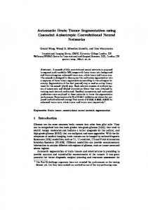
models. Such a system has the possibility of monitoring the fish continuously and build up adequate statistics over time. For this approach to work effectively the same fish within one stereo pair has to be properly segmented. This is a difficult task due to a highly cluttered image background, inhomogeneous lighting and several overlapping objects. Figure 1 shows an example of a medium complex image within a fish cage. The image contains approximately 20 fish and our goal is to segment as many of these as possible. Preferably we would like to segment fish where the complete fish is imaged within the image frame. We will use the image in Fig. 1 as an example image throughout this paper.

Fig. 1. An example of a medium complex image of fish swimming around in a fish cage. Several overlapping fish are observed. In addition the net of the cage is clearly visible, creating a non-trivial background. The lighting is inhomogeneous with background intensities ranging from 90 in the lowest part and up to 255 (saturation) in the upper part. We consider 8-bit monochrome images. The average intensity within a fish will often lie somewhere in between these values, causing a non-trivial region-based segmentation

Due to the high complexity of the images, we have chosen to use a variational segmentation approach, where information about the shape is added to the functional defining the image energy. Variational image segmentation has become increasingly popular during the last years and there exist several approaches towards solving this problem. Some approaches make use of edges [2], whereas others define homogeneity requirements on the statistics of the regions being segmented [3]. In many cases the images contain a lot of noise, the contrast may be low and the background is often highly cluttered. All these effects cause a non trivial behavior of the image energy. To resolve some of these issues various efforts have been made to include prior information about the shape of the objects of interest. In this paper we follow Cremers et al. [4], who have proposed to include information about shape in a modified Mumford-Shah functional. The modified version is a hybrid model combining the external energy of the Mumford-Shah functional with the internal energy of the snakes into one single functional. Following [4], we use an explicit representation of the contour, but instead of using a spline, we represent the contour by a closed polygonal curve. The statistical shape model of a fish is based upon a set of training shapes, all extracted from real images of fish in a semi-automatic manner.

In Section 2 we briefly describe Cremers’ approach. The energy functional including the shape energy is defined together with a description of the minimization process using gradient descent. In addition, we describe a simple initialization procedure that has been proven to work well for the fish segmentation problem. In Section 3 we present several segmentation results for images of varying degree of complexity. Finally, in Section 4 we conclude and discuss possible future improvements of the procedure.

2 Variational Image Segmentation Using Shape Priors In this section we describe the energy functional following Cremers et al. [4]. The image information and shape information are combined into one variational framework. For a given contour C, the energy is defined by

E (u , C ) =Ei (u , C ) + α ⋅ Ec (C ) .

(1)

Here Ei measures how well the contour C and the associated segmentation u approximate the image. The term Ec favors statistically familiar contours by a learning process, where the parameter α defines the relative strength of the shape prior. We refer to [4] and [5] for detailed information about the theory underlying the model and aspects regarding the implementation of the model. 2.1 Image Energy from Polygonal-Based Mumford-Shah Cremers’ modified Mumford-Shah functional for the image energy Ei is given by the following expression [4]:

1 λ2 2 2 f − u dx + ∇u dx + ν ∫ C s2 ds , ( ) ∫ ∫ 2Ω 2 Ω −C 0 1

Ei (u , C ) =

(2)

where f is the input image and u is an approximation of f within the image plane Ω. The image u may be discontinuous across the segmenting contour C. The parameter λ defines the spatial scale on which smoothing is performed. In all the results presented here we have used λ=7. For this value, the diffusion process obtained when minimizing (2) produces a medium smooth image u maintaining some of the local information in the original image. In this way, gradient information is allowed to propagate towards the fish contour. The last term is due to Cremers et al. [4], who replaced the original contour length norm in the Mumford-Shah functional with the squared L2-norm to restrict the contour points from clustering in one place.

2.2 Shape Energy From Gaussian Shape Statistics The explicit representation of the contour allows for a statistical treatment of the different shapes. This is obtained by extracting several training shapes from high contrast images containing non-overlapping fish. The images of the training shapes are binarized and the fish contour is extracted and represented by a polygonal curve. All the training contours are aligned by similarity transformation and cyclic permutation of the contour points. The contour is represented by a polygonal curve z with N points:

z =( x1 , y1 ,..., x N , y N ) . T

(3)

For a given set of training shapes, the distribution of all contours given by (3) is assumed to have a Gaussian shape probability, with µ denoting the mean contour point vector and Σ the regularized covariance matrix [4]:

⎛ 1 ⎞ Ρ( z ) = exp⎜ − ( z − µ ) T Σ −1 ( z − µ ) ⎟ . ⎝ 2 ⎠

(4)

The Gaussian shape probability corresponds to the following energy measure:

1 E c ( z ) = − log(Ρ( z )) + const = − ( z − µ ) T Σ −1 ( z − µ ) . 2

(5)

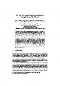
Figure 2 shows 20 training fish used to collect information about the fish shape statistics. All these contours are aligned with respect to similarity transformations and a cyclic permutation of the contour points. Based upon the aligned contours, the mean shape µ and the regularized covariance matrix Σ are extracted.

Fig. 2. 20 fish training shapes extracted from images of real fish. The Gaussian shape statistics is built from these 20 training shapes and incorporated in the Mumford-Shah energy functional.

2.3 Energy Minimization by Gradient Descent We briefly present the resulting evolution equations and refer to Cremers et al. [4,5] for details. Note that the total energy (1) is minimized with respect to both the segmenting contour C and the segmented image u. The Euler-Lagrange equations corresponding to the minimization are then solved by gradient descent. It can be shown that the x-component of the evolution equations for the segmenting contour is given by the following expression

[

]

dxi (t ) = e + ( si , t ) − e − ( si , t ) ⋅ nx ( si , t ) dt + ν ( xi − 2 xi + xi +1 ) − α Σ −1 ( z − µ ) 2i −1.

[

]

(6)

where nx is the x-component of the outer normal vector and the index 2i-1 in the last term is associated with the x-component of contour point number i. e+/- is the energy density in the regions si adjoining the contour C at contour point number i 2

e + / − = ( f − u ) 2 + λ2 ∇u .

(7)

The same equations apply for the y-component of the segmenting contour C. Now, the first term in (6) forces the contour towards the object boundaries. The second term forces equidistant spacing of the contour points, whereas the last term causes a relaxation towards the most probable shape. As pointed out by Cremers et al. [4], the most probable shape is weighted by the inverse of the covariance matrix causing less familiar shape deformations to decay faster. Now, let us turn to the evolution equation for the segmenting image u. Minimizing (1) with respect to the segmenting image u is equivalent to the steady state of the following diffusions process [4]:

∂u 1 = ∇ ⋅ (ωc∇u ) + 2 ( f − u ). ∂t λ

(8)

Here the contour defines a boundary giving rise to an inhomogeneous diffusion process. The indicator function ωc equals zero at the boundary C and one otherwise. Cremers [5] suggested both an explicit finite-difference scheme for (8) and a multigrid method for solving the steady-state equation directly. In this work we use the explicit approximation of (8). 2.4 Automatic Initialization of the Contours The initialization of the contours is of major importance towards a successful segmentation. In this work we have developed a simple algorithm to provide an initial estimate of the segmenting contour. First we locate the potential tails of the fish by

thresholding a low-pass filtered difference image between to consecutive video frames. These consecutive frames are separated 20 ms in time and the motion of the fish usually creates a significant difference between the two frames, especially for the tail region of the fish. This difference is caused by the fish swimming in a direction perpendicular to the edge of the tail. Figure 3 shows the potential tail regions marked with black diamonds in our example image from Fig. 1.

Fig. 3. Potential fish tail candidates marked by black diamonds in our example image from Fig.1. The final initial contours in black and white lines are given by minimizing the projection of the local image orientation along the normal vector of the mean-shape fish µ..

As can be seen from the figure all the true fish tails are correctly located. However, in addition there are quite a few erroneously detected tails related to other parts of the fish or movements of the camera and/or background. All these wrongly classified tails are ruled out by the next step in the initialization process. This step provides a coarse estimate of the size and the rotation of the fish by minimizing the projection of the local image orientation along the normal vectors of the mean-shape fish µ. The projections are obtained by calculating the average scalar product of the fish normal vectors and the local image orientation vectors for several possible fish sizes and angles of rotation. During this process the contour of the mean shape fish is locked to the tail position.

3

Segmentation Results

In this section we present several segmentation results. We start by considering our example image in Fig. 1, where we focus on two different cases.

Figure 4 shows the resulting segmentation of one fish located in the upper left corner of our example image for 4 different initializations of the fish contour. The figure illustrates the sensitivity to the initialization and the problem of the evolving contour being trapped in local minima.

Fig. 4. Segmentation results for one fish in the upper-left corner of the example image in Fig. 1. The images show the final segmentation results (full black lines) for four different contour initializations (dashed black lines). The lower-right plot shows an example of the segmentation process being trapped in a local minimum, where a part of the fish contour is stuck to the edge of a nearby fish.

Figure 5 shows a similar behavior for the large silhouette-like fish in the middle of the example image in Fig. 1. In [4], Cremers et al. discuss the modified Mumford-Shah model and its cartoon limit, which is obtained as λ→∞ in (2). In this case, the diffusion process for u in (8) is replaced by a simple averaging process across the two regions separated by the contour. Thus, the cartoon model is more affected by global gray-level information. Actually, the cartoon model is equally affected by the gray-level information in any part of the image. The cartoon model works poorly for the fish-segmentation problem due to the highly varying gray-level information within both the object and the background. In many cases, the average image intensity inside the fish is similar to the average background intensity causing the segmentation to fail totally. By using the full modified Mumford-Shah model, more local image information is taken into account and in many cases we obtain good segmentation results. This is especially the case for silhouette-like images, where the fish appear dark on a light background. However, the previous two examples show that the segmentation might still fail if the initial contour is too far from the object of interest. Parts of the contour are easily

locked to edges belonging to other fish, thereby causing the segmentation to get trapped in local minima. A good initialization is therefore a prerequisite for a correct segmentation.

Fig. 5. Segmentation results for one fish in the central region of the example image in Fig. 1. The images show the final segmentation results (full white lines) for four different contour initializations (dashed white lines). The lower-right plot shows an example of the segmentation process being trapped in a local minimum, where a part of the fish contour is stuck to the contour of a nearby fish. By increasing the scale parameter λ to 20, a correct segmentation is obtained also for this initialization. For this value of λ the gradient information from the true fish edge is propagated all the way to the fish contour.

The following examples in Fig. 6 show segmentation results on complete images based upon the contour initialization procedure described in Section 2.4. The upper left figure shows the final segmentation result for our example image from Fig. 1. Recall that the initial fish contours for this example image are shown in Fig. 3.

Fig. 6. The figure shows the automatic segmentation results for four different images with a varying degree of complexity. The upper-left image shows the segmentation result for the complete example image from Fig. 1. All the fish are correctly segmented except one of the fish in the bottom part of the image. Here two fish are overlapping almost completely and the segmented fish hiding behind is probably larger than ground truth. In the upper-right image both fish are correctly segmented. The upper fish has a more complex intensity distribution than the silhouette-like fish we have looked at so far. The two lowermost images show examples of automatic segmentation results in rather complex images, where the background is practically similar to the objects of interest. In the lower-left image only one fish has passed the initialization criterion. The segmented contour misses the tail somewhat. In the lower-right image the lowermost fish is correctly segmented. The contour of the uppermost fish misses the upper part of the fish, whereas the contour of the fish in the central region of the image is a bit too small. The rightmost fish seems to be correctly segmented; however, it is hard to tell since half the fish is outside the image frame.

4

Summary and Future Work

We have presented results from a study where we segment fish in images captured within fish cages. Our ultimate goal has been to use this information as part of a stereo-based video surveillance system to extract the weight distribution of the fish within the cages. Statistical shape knowledge was added to the Mumford-Shah functional following Cremers et al. [4]. The fish shape was represented explicitly by a polygonal curve and the energy minimization was done by gradient descent. We obtained good segmentation results for silhouette-like images containing relatively

few fish. In this case, the fish appears dark on a light background and the image energy is well behaved. In cases with more difficult lighting conditions, the contours evolve slowly and often get trapped in local minima. Here the interior of the fish often contains many edges and the image intensity varies in a non-trivial manner. In this case, the Mumford-Shah hypothesis of a piecewise homogeneous gray level value is violated. To improve the existing segmentation, we intend to incorporate local gray-level models for the interior of the fish. In addition, we have the possibility to include motion cues and stereo information to make the segmentation more robust. Moreover, adding balloon forces to the functional (1) could in some cases resolve the problem of the fish contour being locked to nearby edges. Finally, by using more global methods, like graph-cuts and dynamic programming for minimizing the energy, the problem of contours being trapped in local minima should be reduced even further. Acknowledgments. We thank AKVASmart for providing images of fish within fish cages.

References 1.

2. 3. 4. 5.

For more information about an existing stereo system, see: www.akvasmart.com. The AKVA group has developed Vicass – a stereo-based imaging system for size and weight estimation currently used in more than 100 fish farms and distributed and sold in more than eight countries world wide. Kass, M., Witkin, A. and Terzopoulos, D. Snakes: Active contour models. Int. J. of Comp. Vis., 1 (4): 321-331 (1988). Mumford, D., and Shah, J. Optimal Approximations by piecewise smooth functions and associated variational problems. Comm. Pure Appl. Math., 42: 577-685 (1989). Cremers, D., Tischhäuser F., Weickert J., Schnörr C. Diffusion Snakes: Introducing Statistical Shape Knowledge into the Mumford-Shah functional. Int. J. of Comp. Vis., 50 (3), 295-313 (2002). Cremers, D. Statistical Shape Knowledge in Variational Image Segmentation PhD thesis. University of Mannheim (2002)